Survival, Time-to-Event, and Recurrent-Event Models

Prediction surfaces and modeling choices across ExponentialPH, WeibullPH, CoxPH, and Andersen–Gill

This vignette is the richer worked companion to the class reference pages for the survival submodule.

import numpy as np
import pandas as pd
import matplotlib.pyplot as plt
import crabbymetrics as cm

np.set_printoptions(precision=4, suppress=True)

Four estimators, two prediction philosophies

crabbymetrics currently exposes four event-time estimators:

• ExponentialPH: parametric PH with constant baseline hazard,
• WeibullPH: parametric PH with monotone baseline hazard,
• CoxPH: semiparametric proportional hazards,
• AndersenGill: counting-process Cox for recurrent events or split intervals.

The prediction contract differs for a principled reason.

• The parametric PH models identify the baseline hazard, so they can return hazard, cumulative hazard, and survival.
• The Cox-style models leave the baseline hazard unspecified, so the paved prediction object is relative risk.

Simulate a Weibull PH design

rng = np.random.default_rng(20260524)
n = 900
beta_true = np.array([0.55, -0.35])
shape_true = 1.45
scale_hazard_true = 0.035

x = rng.normal(size=(n, 2))
u = rng.uniform(size=n)
event_time = ((-np.log(u)) / (scale_hazard_true * np.exp(x @ beta_true))) ** (1 / shape_true)
censor_time = rng.exponential(35, size=n)
time = np.minimum(event_time, censor_time)
event = (event_time <= censor_time).astype(float)

print({"events": int(event.sum()), "censor_rate": float(1 - event.mean())})

{'events': 682, 'censor_rate': 0.24222222222222223}

Fit the parametric PH models

exp_ph = cm.ExponentialPH()
exp_ph.fit(x, time, event)

weibull = cm.WeibullPH()
weibull.fit(x, time, event)

pd.DataFrame(
    {
        "truth": beta_true,
        "ExponentialPH": exp_ph.summary()["coef"],
        "WeibullPH": weibull.summary()["coef"],
        "Weibull hazard ratio": weibull.summary()["hazard_ratio"],
    },
    index=["x1", "x2"],
)

	truth	ExponentialPH	WeibullPH	Weibull hazard ratio
x1	0.55	0.373986	0.543250	1.721594
x2	-0.35	-0.306631	-0.443975	0.641481

Parametric prediction surfaces

check_x = x[:5]
check_t = np.linspace(2.0, 12.0, 5)

exp_preds = pd.DataFrame(
    {
        "time": check_t,
        "lin": exp_ph.predict_lin(check_x),
        "hazard": exp_ph.predict_hazard(check_x),
        "cumhaz": exp_ph.predict_cumulative_hazard(check_x, check_t),
        "survival": exp_ph.predict(check_x, check_t),
    }
)
exp_preds

	time	lin	hazard	cumhaz	survival
0	2.0	-2.523673	0.080165	0.160329	0.851863
1	4.5	-1.541413	0.214078	0.963352	0.381611
2	7.0	-2.573994	0.076230	0.533613	0.586482
3	9.5	-2.344797	0.095867	0.910733	0.402229
4	12.0	-2.754569	0.063636	0.763638	0.465968

weibull_preds = pd.DataFrame(
    {
        "time": check_t,
        "lin": weibull.predict_lin(check_x, check_t),
        "hazard": weibull.predict_hazard(check_x, check_t),
        "cumhaz": weibull.predict_cumulative_hazard(check_x, check_t),
        "survival": weibull.predict_survival(check_x, check_t),
    }
)
weibull_preds

	time	lin	hazard	cumhaz	survival
0	2.0	-3.060031	0.046886	0.062667	0.939257
1	4.5	-1.234688	0.290926	0.874893	0.416907
2	7.0	-2.513302	0.081000	0.378918	0.684602
3	9.5	-2.027687	0.131640	0.835738	0.433554
4	12.0	-2.506275	0.081572	0.654154	0.519882

The internal identities line up exactly:

{
    "exp hazard = exp(lin)": np.allclose(exp_preds["hazard"], np.exp(exp_preds["lin"])),
    "exp survival = exp(-cumhaz)": np.allclose(exp_preds["survival"], np.exp(-exp_preds["cumhaz"])),
    "weibull hazard = exp(lin)": np.allclose(weibull_preds["hazard"], np.exp(weibull_preds["lin"])),
    "weibull survival = exp(-cumhaz)": np.allclose(weibull_preds["survival"], np.exp(-weibull_preds["cumhaz"])),
}

{'exp hazard = exp(lin)': True,
 'exp survival = exp(-cumhaz)': True,
 'weibull hazard = exp(lin)': True,
 'weibull survival = exp(-cumhaz)': True}

Cox proportional hazards

cox = cm.CoxPH()
cox.fit(x, time, event)

cox_table = pd.DataFrame(
    {
        "truth": beta_true,
        "coef": cox.summary()["coef"],
        "hazard ratio": cox.summary()["hazard_ratio"],
        "se": cox.summary()["se"],
    },
    index=["x1", "x2"],
)
cox_table

	truth	coef	hazard ratio	se
x1	0.55	0.540299	1.716519	0.044353
x2	-0.35	-0.440718	0.643574	0.042970

Since the baseline hazard is left unspecified, the default prediction is relative risk rather than absolute survival:

cox_preds = pd.DataFrame(
    {
        "log_hazard_ratio": cox.predict_lin(check_x),
        "relative_risk": cox.predict(check_x),
    }
)
cox_preds

	log_hazard_ratio	relative_risk
0	-0.335467	0.715004
1	1.077264	2.936634
2	-0.411353	0.662753
3	-0.078487	0.924514
4	-0.669401	0.512015

Andersen–Gill for recurrent events or split intervals

A convenient smoke test is to split each subject into two rows with the event, if any, carried only by the final interval.

start_long = np.concatenate([np.zeros_like(time), time / 2])
stop_long = np.concatenate([time / 2, time])
x_long = np.vstack([x, x])
event_long = np.concatenate([np.zeros_like(event), event])

ag = cm.AndersenGill()
ag.fit(x_long, start_long, stop_long, event_long)

pd.DataFrame(
    {
        "CoxPH": cox.summary()["coef"],
        "Andersen-Gill split rows": ag.summary()["coef"],
    },
    index=["x1", "x2"],
)

	CoxPH	Andersen-Gill split rows
x1	0.540299	0.540299
x2	-0.440718	-0.440718

ag_preds = pd.DataFrame(
    {
        "log_hazard_ratio": ag.predict_lin(check_x),
        "relative_risk": ag.predict(check_x),
    }
)
ag_preds

	log_hazard_ratio	relative_risk
0	-0.335467	0.715004
1	1.077264	2.936634
2	-0.411353	0.662753
3	-0.078487	0.924514
4	-0.669401	0.512015

Visualizing survival curves from the parametric fit

grid = np.linspace(0.1, np.quantile(time, 0.9), 100)
profiles = np.array([
    [0.0, 0.0],
    [1.0, 0.0],
    [0.0, 1.0],
])
labels = ["x=(0,0)", "x=(1,0)", "x=(0,1)"]

fig, ax = plt.subplots(figsize=(7, 4.5))
for profile, label in zip(profiles, labels):
    xx = np.tile(profile, (len(grid), 1))
    ax.plot(grid, weibull.predict_survival(xx, grid), label=label)

ax.set_xlabel("time")
ax.set_ylabel("estimated survival")
ax.set_title("WeibullPH survival curves")
ax.legend(frameon=False)
plt.show()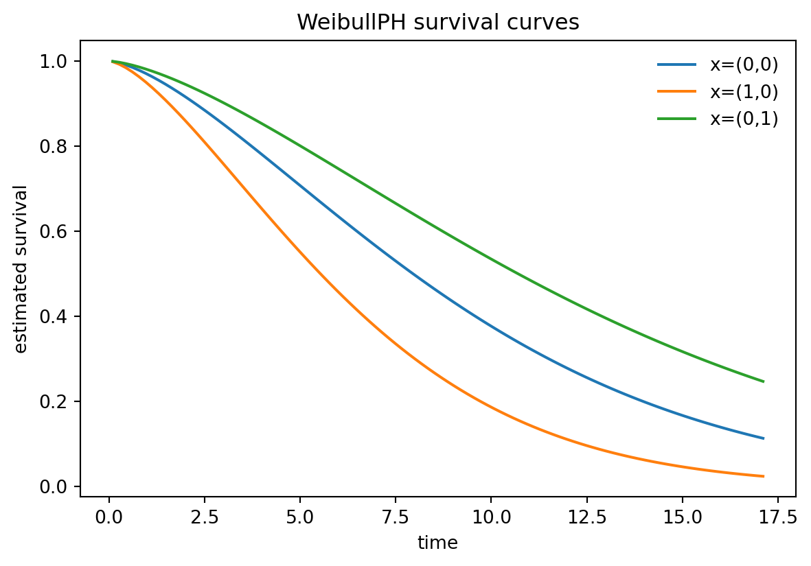

Interpretation

The current survival module has a clean split:

• parametric PH models for absolute event-time prediction,
• Cox-style models for semiparametric relative-risk estimation,
• Andersen–Gill when the data are naturally in risk-interval form.

That division is what drives the prediction API. The model returns the richest object it can justify from the fitted likelihood or partial likelihood.