Code
import numpy as np
import pandas as pd
import matplotlib.pyplot as plt
import crabbymetrics as cm

np.set_printoptions(precision=3, suppress=True)Exponential, Weibull, Cox PH, Andersen–Gill, and discrete-time hazards
Survival models describe event timing through a hazard rate: the instantaneous event risk among units still at risk. crabbymetrics includes four first-pass survival estimators:
ExponentialPH: a parametric proportional-hazards model with constant baseline hazard,WeibullPH: a parametric proportional-hazards model with monotone baseline hazard,CoxPH: Cox’s semiparametric proportional-hazards partial likelihood,AndersenGill: the counting-process Cox model for recurrent events or time-split risk intervals.The common coefficient interpretation is multiplicative on the hazard. If a coefficient is \(\beta_j\), then \(\exp(\beta_j)\) is a hazard ratio.
import numpy as np
import pandas as pd
import matplotlib.pyplot as plt
import crabbymetrics as cm
np.set_printoptions(precision=3, suppress=True)The simplest survival observation is one unit followed from a well-defined origin until either an event happens or follow-up stops. For subject \(i\), the latent event time is \(T_i\) and the censoring time is \(C_i\). With ordinary right censoring, the observed record is
\[ Y_i = \min(T_i, C_i), \qquad \Delta_i = \mathbf{1}\{T_i \le C_i\}. \]
So a row contains at least:
Right censoring means we know the event did not occur before \(Y_i\), but we do not know when it would have occurred after \(Y_i\). This is the common setup for attrition, end-of-study censoring, or administrative follow-up windows. The standard identifying condition is independent censoring: conditional on covariates, censoring should not reveal extra information about the event time beyond the fact that the unit survived to the censoring time.
Sometimes units only become observable after an entry time \(L_i\). This is left truncation, or delayed entry: a subject is included only if \(T_i > L_i\). The observation is then a risk interval \((L_i, Y_i]\) plus the event flag \(\Delta_i\). Left truncation changes the risk sets because the subject should not count as being at risk before \(L_i\). This differs from left censoring, where the event is known to have occurred before some time but the exact time is unknown. This vignette focuses on right censoring and, later, interval-style risk sets that can also represent delayed entry or recurrent-event data.
The basic survival objects are:
\[ S(t) = \Pr(T > t), \qquad h(t) = \lim_{\Delta t \downarrow 0} \frac{\Pr(t \le T < t + \Delta t \mid T \ge t)}{\Delta t}, \qquad H(t) = \int_0^t h(u)\,du. \]
Survival and cumulative hazard are linked by
\[ S(t) = \exp\{-H(t)\}. \]
Before fitting regressions, the Kaplan–Meier estimator is the workhorse nonparametric estimate of the survival curve under right censoring. At each distinct observed event time \(t_j\), let \(d_j\) be the number of events at that time and \(n_j\) the number of units still at risk just before that time. The estimator multiplies the conditional survival probabilities across event times:
\[ \widehat S(t) = \prod_{t_j \le t} \left(1 - \frac{d_j}{n_j}\right). \]
Censored observations do not create downward jumps in the curve. They simply leave the risk set after their censoring time. That is the key intuition: Kaplan–Meier estimates survival by using only units that are still genuinely under observation at each failure time.
The Nelson–Aalen cumulative-hazard estimator is the companion object:
\[ \widehat H(t) = \sum_{t_j \le t} \frac{d_j}{n_j}. \]
Regression models below can be read as structured ways to let covariates shift hazards and survival curves, while preserving the same risk-set logic.
Generate a Weibull proportional-hazards design with two covariates. The event time satisfies
\[ H_i(t) = \lambda t^\rho \exp(x_i'\beta), \qquad S_i(t) = \exp\{-H_i(t)\}. \]
Here \(\rho > 1\) gives an increasing baseline hazard. Independent censoring creates the observed time and event indicator.
rng = np.random.default_rng(20260524)
n = 900
beta_true = np.array([0.55, -0.35])
shape_true = 1.45
scale_hazard_true = 0.035

x = rng.normal(size=(n, 2))
u = rng.uniform(size=n)
event_time = ((-np.log(u)) / (scale_hazard_true * np.exp(x @ beta_true))) ** (1 / shape_true)
censor_time = rng.exponential(35, size=n)
time = np.minimum(event_time, censor_time)
event = (event_time <= censor_time).astype(float)

print({"events": int(event.sum()), "censor_rate": float(1 - event.mean())})
{'events': 682, 'censor_rate': 0.24222222222222223}A quick Kaplan–Meier curve from the simulated data shows the raw survival pattern before imposing a regression model. The step function drops only at observed event times; censored units affect later denominators by leaving the risk set.
def kaplan_meier(times, events):
    event_times = np.sort(np.unique(times[events == 1]))
    surv = []
    s = 1.0
    for tj in event_times:
        at_risk = np.sum(times >= tj)
        failures = np.sum((times == tj) & (events == 1))
        s *= 1 - failures / at_risk
        surv.append((tj, s, at_risk, failures))
    return pd.DataFrame(surv, columns=["time", "survival", "at_risk", "events"])

km = kaplan_meier(time, event)
km.head()| time | survival | at_risk | events | |
|---|---|---|---|---|
| 0 | 0.013369 | 0.998885 | 897 | 1 |
| 1 | 0.064539 | 0.997768 | 894 | 1 |
| 2 | 0.130955 | 0.996648 | 891 | 1 |
| 3 | 0.159742 | 0.995528 | 890 | 1 |
| 4 | 0.237237 | 0.994405 | 886 | 1 |
fig, ax = plt.subplots(figsize=(7, 4.2))
ax.step(np.r_[0, km["time"]], np.r_[1, km["survival"]], where="post")
ax.set_xlabel("time")
ax.set_ylabel("Kaplan--Meier survival estimate")
ax.set_title("Nonparametric survival curve for the simulated sample")
ax.set_ylim(0, 1.02)
plt.show()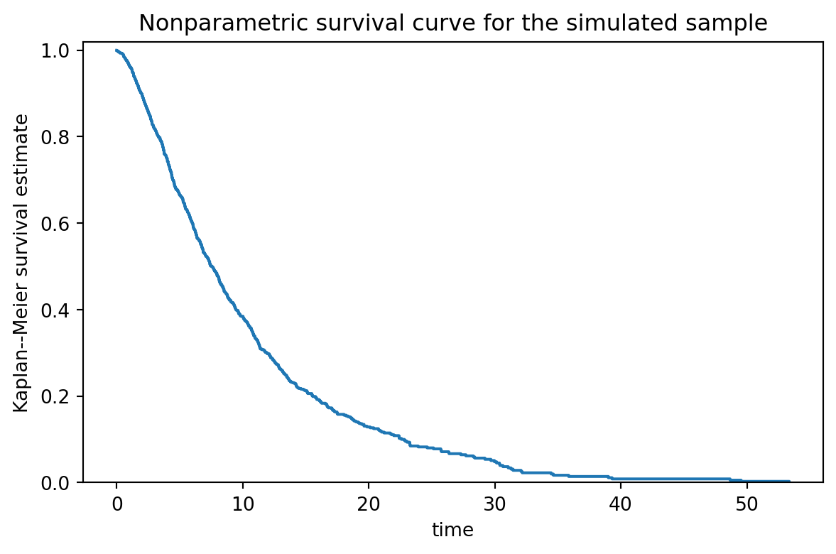
The exponential model is the special case \(\rho = 1\):
\[ h_i(t) = \lambda \exp(x_i'\beta), \qquad H_i(t) = \lambda t \exp(x_i'\beta). \]
The Weibull model estimates \(\rho\) too:
\[ h_i(t) = \lambda \rho t^{\rho - 1}\exp(x_i'\beta), \qquad H_i(t) = \lambda t^\rho\exp(x_i'\beta). \]
exp_ph = cm.ExponentialPH()
exp_ph.fit(x, time, event)

weibull = cm.WeibullPH()
weibull.fit(x, time, event)

parametric = pd.DataFrame(
    {
        "truth": [beta_true[0], beta_true[1], shape_true],
        "exponential": [*exp_ph.summary()["coef"], np.nan],
        "weibull": [*weibull.summary()["coef"], weibull.summary()["shape"]],
    },
    index=["x1 log hazard ratio", "x2 log hazard ratio", "Weibull shape"],
)
parametric| truth | exponential | weibull | |
|---|---|---|---|
| x1 log hazard ratio | 0.55 | 0.373986 | 0.543250 |
| x2 log hazard ratio | -0.35 | -0.306631 | -0.443975 |
| Weibull shape | 1.45 | NaN | 1.496373 |
The exponential fit is intentionally misspecified because the simulated baseline hazard is not constant. The log-hazard-ratio coefficients remain in the right neighborhood, while the Weibull fit also recovers an increasing baseline hazard.
The widened survival API now exposes the same layered contract as the MLE estimators:
predict_lin(...): the linear predictor on the model’s natural latent scale,predict(...): the default mean-scale prediction,predict_hazard(...), predict_cumulative_hazard(...), and predict_survival(...) when absolute survival objects are identified.For the parametric PH models, predict(...) defaults to survival probabilities at supplied horizons.
check_x = x[:5]
check_t = np.linspace(2.0, 12.0, 5)

exp_preds = pd.DataFrame(
    {
        "time": check_t,
        "lin": exp_ph.predict_lin(check_x),
        "hazard": exp_ph.predict_hazard(check_x),
        "cumhaz": exp_ph.predict_cumulative_hazard(check_x, check_t),
        "survival": exp_ph.predict(check_x, check_t),
    }
)
exp_preds| time | lin | hazard | cumhaz | survival | |
|---|---|---|---|---|---|
| 0 | 2.0 | -2.523673 | 0.080165 | 0.160329 | 0.851863 |
| 1 | 4.5 | -1.541413 | 0.214078 | 0.963352 | 0.381611 |
| 2 | 7.0 | -2.573994 | 0.076230 | 0.533613 | 0.586482 |
| 3 | 9.5 | -2.344797 | 0.095867 | 0.910733 | 0.402229 |
| 4 | 12.0 | -2.754569 | 0.063636 | 0.763638 | 0.465968 |
weibull_preds = pd.DataFrame(
    {
        "time": check_t,
        "lin": weibull.predict_lin(check_x, check_t),
        "hazard": weibull.predict_hazard(check_x, check_t),
        "cumhaz": weibull.predict_cumulative_hazard(check_x, check_t),
        "survival": weibull.predict_survival(check_x, check_t),
    }
)
weibull_preds| time | lin | hazard | cumhaz | survival | |
|---|---|---|---|---|---|
| 0 | 2.0 | -3.060031 | 0.046886 | 0.062667 | 0.939257 |
| 1 | 4.5 | -1.234688 | 0.290926 | 0.874893 | 0.416907 |
| 2 | 7.0 | -2.513302 | 0.081000 | 0.378918 | 0.684602 |
| 3 | 9.5 | -2.027687 | 0.131640 | 0.835738 | 0.433554 |
| 4 | 12.0 | -2.506275 | 0.081572 | 0.654154 | 0.519882 |
The internal identities line up exactly:
np.allclose(exp_preds["hazard"], np.exp(exp_preds["lin"]))Truenp.allclose(exp_preds["survival"], np.exp(-exp_preds["cumhaz"]))Truenp.allclose(weibull_preds["hazard"], np.exp(weibull_preds["lin"]))Truenp.allclose(weibull_preds["survival"], np.exp(-weibull_preds["cumhaz"]))TrueThe Cox model leaves the baseline hazard unspecified and estimates \(\beta\) from the ordering of failures through the partial likelihood:
\[ \ell(\beta) = \sum_{i: d_i = 1} \left[x_i'\beta - \log\left\{\sum_{j: t_j \ge t_i}\exp(x_j'\beta)\right\}\right]. \]
cox = cm.CoxPH()
cox.fit(x, time, event)

cox_table = pd.DataFrame(
    {
        "truth": beta_true,
        "CoxPH coef": cox.summary()["coef"],
        "hazard ratio": cox.summary()["hazard_ratio"],
        "se": cox.summary()["se"],
    },
    index=["x1", "x2"],
)
cox_table| truth | CoxPH coef | hazard ratio | se | |
|---|---|---|---|---|
| x1 | 0.55 | 0.540299 | 1.716519 | 0.044353 |
| x2 | -0.35 | -0.440718 | 0.643574 | 0.042970 |
For Cox, the default prediction is relative risk because the baseline hazard is left unspecified. The latent score is the log hazard ratio.
cox_preds = pd.DataFrame(
    {
        "log_hazard_ratio": cox.predict_lin(check_x),
        "relative_risk": cox.predict(check_x),
    }
)
cox_preds| log_hazard_ratio | relative_risk | |
|---|---|---|
| 0 | -0.335467 | 0.715004 |
| 1 | 1.077264 | 2.936634 |
| 2 | -0.411353 | 0.662753 |
| 3 | -0.078487 | 0.924514 |
| 4 | -0.669401 | 0.512015 |
Andersen–Gill is the Cox partial likelihood with risk intervals \((s_i, t_i]\) instead of one row per subject. A row is in the risk set for an event at time \(t\) when
\[ s_i < t \le t_i. \]
That makes the model useful for recurrent events and time-varying covariates. As a smoke test, split each original subject into two rows with unchanged covariates; only the second row can carry the original terminal event. The Andersen–Gill estimate then agrees with the ordinary Cox estimate.
start_long = np.concatenate([np.zeros_like(time), time / 2])
stop_long = np.concatenate([time / 2, time])
x_long = np.vstack([x, x])
event_long = np.concatenate([np.zeros_like(event), event])

ag = cm.AndersenGill()
ag.fit(x_long, start_long, stop_long, event_long)

pd.DataFrame(
    {
        "CoxPH": cox.summary()["coef"],
        "Andersen-Gill split rows": ag.summary()["coef"],
    },
    index=["x1", "x2"],
)| CoxPH | Andersen-Gill split rows | |
|---|---|---|
| x1 | 0.540299 | 0.540299 |
| x2 | -0.440718 | -0.440718 |
ag_preds = pd.DataFrame(
    {
        "log_hazard_ratio": ag.predict_lin(check_x),
        "relative_risk": ag.predict(check_x),
    }
)
ag_preds| log_hazard_ratio | relative_risk | |
|---|---|---|
| 0 | -0.335467 | 0.715004 |
| 1 | 1.077264 | 2.936634 |
| 2 | -0.411353 | 0.662753 |
| 3 | -0.078487 | 0.924514 |
| 4 | -0.669401 | 0.512015 |
Parametric models estimate an absolute survival curve because they estimate the baseline hazard. Cox-type partial-likelihood models estimate relative hazards unless a baseline-hazard estimator is added.
grid = np.linspace(0.1, np.quantile(time, 0.9), 100)
profiles = np.array([
    [0.0, 0.0],
    [1.0, 0.0],
    [0.0, 1.0],
])
labels = ["x=(0,0)", "x=(1,0)", "x=(0,1)"]

fig, ax = plt.subplots(figsize=(7, 4.5))
for profile, label in zip(profiles, labels):
    xx = np.tile(profile, (len(grid), 1))
    ax.plot(grid, weibull.predict_survival(xx, grid), label=label)

ax.set_xlabel("time")
ax.set_ylabel("estimated survival")
ax.set_title("WeibullPH survival curves")
ax.legend(frameon=False)
plt.show()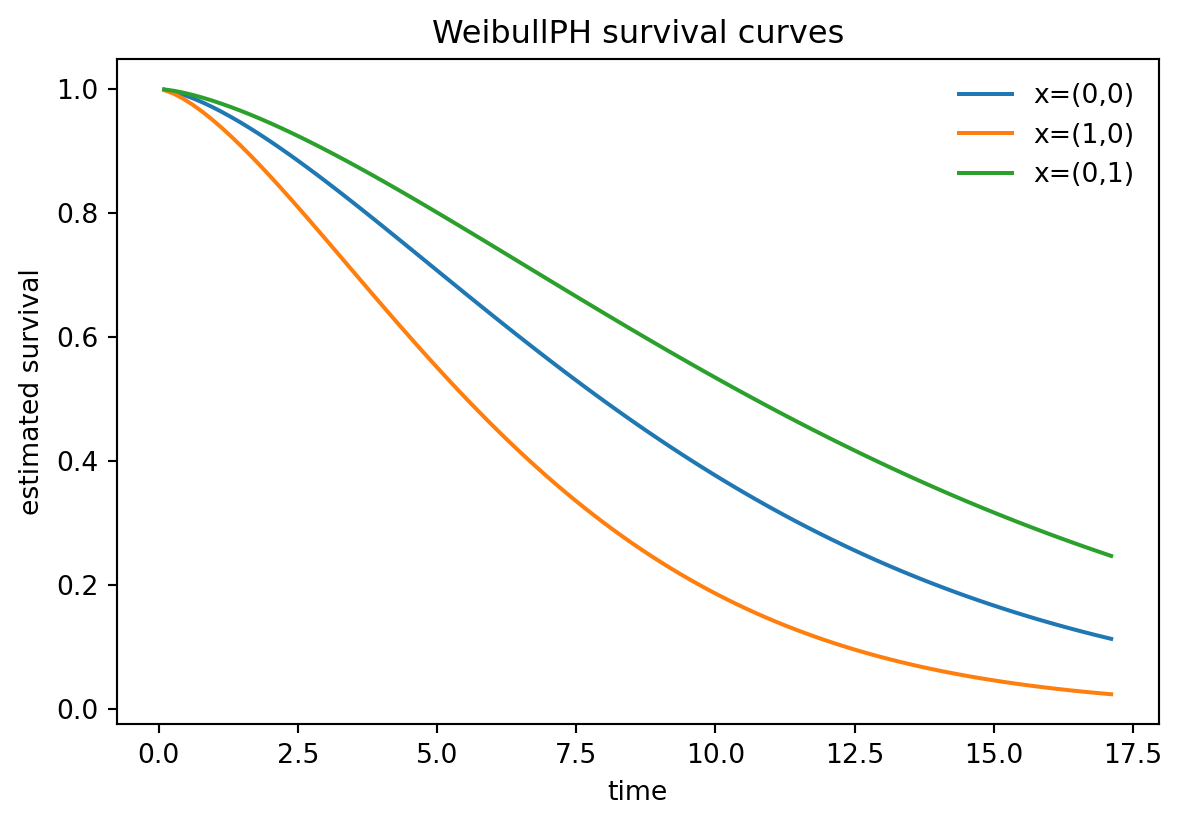
A continuous-time survival record can be expanded into person-period rows. For subject \(i\) and interval \(k\), define \(Y_{ik}=1\) if the event occurs in that interval and \(0\) if the subject survives the interval. Conditional on being at risk at the start of the interval,
\[ \Pr(Y_{ik}=1 \mid Y_{i1}=\cdots=Y_{i,k-1}=0, x_i) = h_{ik}. \]
A pooled binary regression on person-period rows is therefore a discrete-time hazard model. With a logit link,
\[ \operatorname{logit}(h_{ik}) = \alpha_k + x_i'\beta, \]
where the interval dummies \(\alpha_k\) are the discrete baseline hazard. The survival function through interval \(K\) is the product of conditional survival probabilities:
\[ S_i(K) = \prod_{k=1}^K (1 - h_{ik}). \]
This is the same factorization that underlies grouped-duration likelihoods. If the interval event probabilities are small, the complementary-log-log link is especially close to a continuous-time proportional-hazards model because
\[ \log\{-\log(1-h_{ik})\} = \alpha_k + x_i'\beta \]
corresponds to a piecewise-constant baseline cumulative hazard. The logit link is not identical to Cox PH, but it is a very useful discrete-time analog: the regression is on the sequence of conditional hazards rather than on a one-shot outcome.
If we aggregate person-period rows within cells, say by interval and covariate group, we observe \(y_g\) events out of \(m_g\) risk-set trials. A plain grouped discrete-time hazard model treats
\[ y_g \sim \operatorname{Binomial}(m_g, h_g), \qquad \operatorname{logit}(h_g)=z_g'\theta. \]
A beta-binomial version adds extra-binomial heterogeneity by letting the cell hazard vary around its mean:
\[ p_g \sim \operatorname{Beta}(a_g, b_g), \qquad Y_g \mid p_g \sim \operatorname{Binomial}(m_g, p_g). \]
That is a grouped, overdispersed discrete-time survival model. It is useful when subjects in the same interval/cell have unmodeled frailty or shared shocks, so the event counts are more variable than a binomial hazard would imply. In that sense:
Here is the person-period construction with a few interval dummies. The coefficient should have the same sign as the Cox and Weibull estimates, though the scale is log-odds of interval failure rather than log instantaneous hazard.
breaks = np.quantile(time, np.linspace(0, 0.85, 9))
breaks[0] = 0.0
rows = []
for i in range(n):
    for k in range(len(breaks) - 1):
        left, right = breaks[k], breaks[k + 1]
        if time[i] <= left:
            break
        at_risk_width = min(time[i], right) - left
        if at_risk_width <= 0:
            continue
        yik = float(event[i] == 1 and time[i] <= right)
        rows.append((yik, k, x[i, 0], x[i, 1]))
        if yik == 1 or time[i] <= right:
            break

pp = pd.DataFrame(rows, columns=["event", "interval", "x1", "x2"])
interval = pd.get_dummies(pp["interval"].astype(int), prefix="t", drop_first=True).astype(float)
X_logit = np.column_stack([pp[["x1", "x2"]].to_numpy(), interval.to_numpy()])
y_logit = pp["event"].to_numpy().astype(np.int32)

logit = cm.Logit(alpha=0.0, max_iterations=500, gradient_tolerance=1e-7)
logit.fit(X_logit, y_logit)

pd.DataFrame(
    {
        "Cox log hazard ratio": cox.summary()["coef"],
        "person-period logit coefficient": logit.summary()["coef"][:2],
    },
    index=["x1", "x2"],
)| Cox log hazard ratio | person-period logit coefficient | |
|---|---|---|
| x1 | 0.540299 | -0.584777 |
| x2 | -0.440718 | 0.467736 |
The equality is conceptual rather than literal: logit coefficients live on the discrete interval-failure odds scale, while Cox and Weibull coefficients live on the instantaneous hazard scale. With short intervals and rare failures per interval, they often tell the same directional story.