Gaussian splatting: representation, rendering and fitting
Gaussian splatting represents an image or scene using overlapping Gaussian-shaped primitives. A renderer projects and blends these primitives into pixels. Their parameters can be learned by comparing renders with photographs. gsplat supplies fast differentiable rendering operations; it does not itself invent a 3D object from a text prompt.
Start with the two-dimensional version used here, then add camera projection to understand genuine 3D Gaussian splatting.
1. A Gaussian footprint
Let $u=(u_x,u_y)^\top$ denote a pixel location. Splat $i$ has centre $\mu_i\in\mathbb R^2$ and positive-definite covariance $\Sigma_i$. Its footprint is
It is largest at the centre and decreases smoothly with distance. Its level sets are ellipses. Two radii and a rotation determine their shape:
This is not a normalized probability density: there is no determinant or $2\pi$ normalizing factor. It describes the spatial falloff of opacity.
A single red splat on a light background. Radii are measured along its own axes before rotation. The outline is the two-radius contour.
2. Opacity and colour compositing
A splat also has colour $c_i\in[0,1]^3$ and peak opacity $o_i\in[0,1]$. Its opacity at pixel $u$ is $\alpha_i(u)=o_i g_i(u)$. Rendering normally uses front-to-back alpha compositing, not an unweighted sum of colours. For an ordered list of splats, define the light transmitted before splat $i$:
Including background colour $b$, the pixel is
For example, put a red splat of opacity 0.6 in front of a green one of opacity 0.5, against black. The pixel receives 0.6 red and $0.4\times0.5=0.2$ green. Reversing their order gives 0.3 red and 0.5 green. Order therefore matters. Practical rasterizers truncate tiny contributions and clamp alpha for efficiency and numerical stability.
3. Fitting the photograph
Here, $\Theta$ contains nine real numbers per splat: two centre coordinates, two log-radii, one angle, three colour logits and one opacity logit. Exponentials keep radii positive; logistic transforms keep colour and opacity in the unit interval. For target image $I$ of width $W$ and height $H$, the objective is
The renderer differentiates pixel values with respect to the splat parameters. Backpropagation supplies $\nabla_\Theta\mathcal L$, and Adam updates the parameters. This is a nonconvex problem: initialization, step sizes and the optimization budget affect the result.
Roughly 80% of centres start on a grid; the remainder are sampled preferentially near image detail. Initial colours come from the photo. Every model gets 5,000 steps with the same objective and seed. The position learning rate and scale bounds adapt to the initial spacing, allowing small models to use broad splats. This is direct fitting, not pretrained semantic understanding.
4. Splat count versus matrix rank
Increasing $N$ adds adjustable primitives. This planar model has $9N$ trainable scalars: 64 splats use 576; 24,000 use 216,000. That measures capacity, but it is not the rank of the image matrix.
A rank-$r$ matrix approximation uses a sum of $r$ outer products with a linear-algebraic rank bound. Splats instead have localized, rotated footprints with learned positions, and opacity-dependent compositing. The rotated footprints and transmittance products do not impose a corresponding rank-$N$ bound. This is closer to a learned nonlinear basis representation.
Small models use broad ellipses for dominant colours and shapes. Larger models can allocate smaller footprints to eyes, lettering and texture. These models are independent fits, not nested subsets. Extra capacity offers flexibility, but does not guarantee better finite-iteration optimization or generalization.
5. Extension to 3D scenes
A 3D Gaussian has centre $m_i\in\mathbb R^3$ and covariance $\Sigma_i^{3D}=Q_i\operatorname{diag}(s_{1i}^2,s_{2i}^2,s_{3i}^2)Q_i^\top$, where $Q_i$ is a 3D rotation. A calibrated camera transforms its centre to $(X,Y,Z)$ and projects it:
Under the standard local-affine approximation, the screen-space centre is $\pi(m_i^{\rm cam})$, and the covariance is approximately
Here $R_{\rm cam}$ is the camera rotation, $J_i$ is the Jacobian of the perspective projection at that Gaussian’s camera-space centre, and $\varepsilon I_2$ adds a small footprint for rasterization stability. The projected splats are depth-ordered and composited.
Many 3DGS systems use spherical harmonics for view-dependent colour and adapt the number of splats through splitting, cloning and pruning. Meaningful scene reconstruction normally uses several photographs with known or estimated camera poses; COLMAP can supply poses and an initial point cloud. Different views constrain where a splat can be in space.
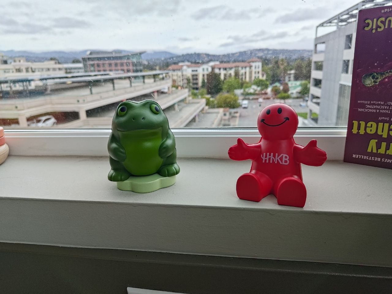
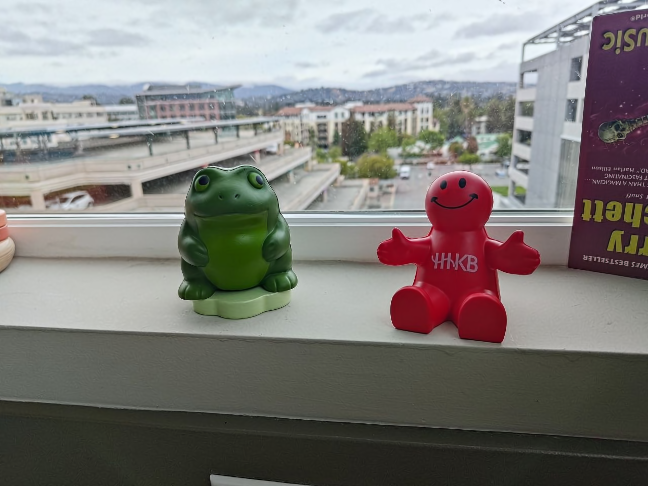
Our demonstration uses the 3D rasterizer but fixes all centres at the same depth, gives them negligible thickness and permits only in-plane rotation. It is effectively a planar image representation. A close pixel match does not recover the frog’s shape, identify depth, or reveal hidden surfaces.
6. Measuring approximation error
For RGB values scaled to $[0,1]$, peak signal-to-noise ratio is
A gain of about 3 dB halves squared pixel error. PSNR does not directly measure perceptual quality, geometry or held-out performance. The displayed metric uses the unquantized renderer output; the downloadable 8-bit PNG adds a small quantization error.
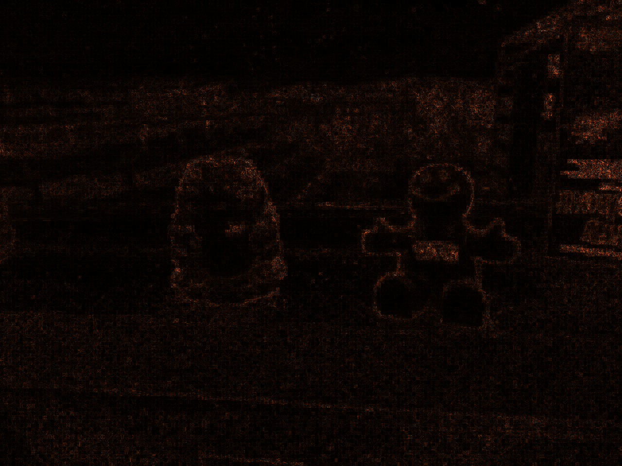
The Difference view shows mean absolute RGB error at each pixel, multiplied by eight on the same scale for every model. It does not rescale each image to look equally bright.
Sources and implementation
- Ye et al. (2025), gsplat: An Open-Source Library for Gaussian Splatting.
- Kerbl et al. (2023), 3D Gaussian Splatting for Real-Time Radiance Field Rendering.
- Fitting source and parameter-only re-rendering source. The photo is not needed to render a saved model.