Minimum-Distance Estimation on a Cohort-by-Event-Time Lattice
Author
Apoorva Lal
Published
July 16, 2026
Abstract
Staggered-adoption event studies present an unresolved bias-variance tradeoff. A pooled event-study regression is precise and can fail to estimate an interpretable average treatment-effect curve when effects differ across adoption cohorts. A saturated cohort-by-event-time estimator accommodates that heterogeneity and can be noisy when there are many small cohorts. This paper proposes an adaptive estimator between those endpoints. Starting from a saturated heterogeneity-robust estimate, we construct minimum-distance projections onto a nested lattice of adjacent cohort and event-time partitions. Every candidate estimates the same support-aware aggregate event-study curve. A Lepskii rule selects the lowest-dimensional candidate whose curve agrees statistically with every finer comparable model. Cross-model covariance and a simultaneous critical value are obtained from the saturated regression’s cluster influence functions. Hyperparameter grids are tuned by honest nested cluster splitting against an independent saturated target estimate. Simulations with nine uneven adoption cohorts show that the selector recovers cohort-only, time-only, and tensor-product structure while approaching saturation when pooling distorts the target. The method is implemented as a pyfixest-compatible Python class.
1. Introduction
The recent difference-in-differences literature has clarified why a conventional two-way fixed-effects (TWFE) event study can fail to estimate a meaningful average of heterogeneous treatment effects under staggered adoption (Goodman-Bacon 2021; Chaisemartin and D’Haultfœuille 2020; Goldsmith-Pinkham, Hull, and Kolesár 2024). A direct response is to estimate treatment effects separately for every adoption cohort and event time, then aggregate the resulting cells using transparent nonnegative weights (Sun and Abraham 2021; Callaway and Sant’Anna 2021; Wooldridge 2021). That response protects the estimand and introduces a potentially large collection of noisy cohort-time coefficients.
This paper treats the choice between pooled and saturated event studies as an adaptive estimation problem. The motivating joint-test approach in Lal (2025) asks whether cohort-specific deviations from a common event-study curve are jointly zero. The test supplies a useful binary diagnostic. Rejection leaves the appropriate degree of partial pooling unresolved, and nonrejection leaves the magnitude of pooling bias unresolved. The resulting estimation problem is to determine how much structured heterogeneity the data can support.
The selection logic follows Lepskii’s comparison-to-refinement principle (Lepski 1990; Lepski and Spokoiny 1997; Goldenshluger and Lepski 2011). It is also related to recent work on adaptation to misspecification, where efficiency gains from a restricted model are weighed against detectable departures from that model (Armstrong, Kline, and Sun 2025). Our setting differs because the candidate class is a two-dimensional partial order and every model must be mapped to the same dynamic treatment-effect target.
We propose a two-axis partial-pooling estimator. The first axis groups adjacent adoption cohorts. The second groups adjacent event times, while preserving the pre/post boundary. Crossing the two partitions produces rectangular restrictions on the cohort-by-event-time treatment-effect surface. The coarsest candidates have a few interpretable blocks; the finest candidate is saturated. All candidates are linear minimum-distance projections of one saturated estimate, and all are mapped to the same support-aware aggregate event-study target.
The estimator has three useful features. First, one expensive fixed-effects regression produces the entire candidate path. Second, because every candidate is a linear transformation of the same saturated estimator, cross-model covariance is available exactly from a shared influence-function stack. Third, a cluster multiplier bootstrap can calibrate one critical value simultaneously over candidate models, refinements, and event times.
The paper makes four contributions.
It formulates partial pooling over a nested cohort-time lattice while holding the reported event-study estimand fixed.
It derives the minimum-distance candidate estimators and their joint covariance from a saturated heterogeneity-robust fit.
It gives a Lepskii selection rule and an honest nested-splitting procedure for tuning the candidate grid without using final-sample performance.
It implements the procedure in Python and evaluates risk, oracle regret, coverage, selection, and computation in a repeated many-cohort experiment.
The selected complexity pertains to a particular aggregate target. Distinct cohort effects may cancel under that target, making pooling useful for the aggregate curve while leaving the latent surface heterogeneous. Claims about full-surface homogeneity require a surface-level selection criterion. This distinction is central to interpreting the results.
2. Setup and Target
The introduction motivates a bias-variance tradeoff whose solution requires all candidate estimators to answer the same causal question. This section fixes that question, records which cohort-event cells are supported, and defines the saturated heterogeneity-robust estimator from which every later candidate is constructed. Its outputs are the base coefficient vector \hat\theta, covariance \hat\Sigma, influence contributions \hat\psi_c, and target map L used by the adaptive method in Section 3.
2.1 Staggered adoption
Units i=1,\ldots,n are observed in periods t=1,\ldots,T. Treatment adoption is absorbing:
D_{it}=1\{t\geq G_i\},
where G_i\in\mathcal G\cup\{\infty\} is the adoption date and G_i=\infty denotes a never-treated unit. Event time is s=t-G_i. Let \mathcal G_T=\{g_1<\cdots<g_J\} denote treated cohorts and let \mathcal S denote the reported event-time window, excluding the normalized reference period s=-1.
We maintain no anticipation, parallel trends for untreated potential outcomes, and overlap for every reported cell. The current implementation uses never-treated observations as the comparison group in a saturated interaction regression. The minimum-distance construction applies without change when the base vector and influence functions come from another identified heterogeneity-robust estimator.
2.2 Supported cells
Let \mathcal I\subseteq\mathcal G_T\times\mathcal S be the set of estimable cells. A cell enters \mathcal I only when it reaches a prespecified minimum support and the saturated design retains its coefficient. Unsupported cells receive zero target weight, and the remaining weights are renormalized over supported cohorts at each event time. This exposes the changing target population and prevents extrapolation of late event times for late adopters.
Stack supported effects in \theta\in\mathbb R^p. The reported dynamic ATT is
Post-treatment observations beyond the reporting window are trimmed, isolating the fixed effects from unmodeled tail effects. Earlier leads remain in the estimation sample under no anticipation. Let \hat\theta be the retained saturated coefficient vector and \hat\Sigma its cluster-robust covariance.
We assume the finite-dimensional asymptotic linear representation
where c indexes independent clusters. The scaling is absorbed into \hat\psi_c. In pyfixest, these contributions are constructed from the cluster sums of residualized regressor scores and the regression bread.
2.4 The estimator in miniature
Consider three adoption cohorts and three post-treatment event times. Suppress one lead period, which remains in its own block throughout the example and is included in each E count below. Figure 1 places the saturated cell estimates beside the weights used to form the aggregate target.
Figure 1: A miniature saturated effect surface and its event-time-specific target weights. Clustered standard errors are 0.35 for the early and middle cohorts and 0.45 for the late cohort. Interactive tooltips report the estimate, standard error, and target weight in every cell.
The left panel has an evident low-dimensional pattern: the early and middle cohorts are similar, their first two effects are nearly flat, and the late cohort follows a different path. The right panel shows why cohort structure can matter for the aggregate curve. The late cohort receives 50 percent of the weight at s=0 and 10 percent at s=2. Applying the displayed weights gives
\hat\tau_{\mathrm{sat}}=(1.73,\ 1.48,\ 1.92).
Figure 2 puts four restrictions on a refinement ladder. C1-E2 uses one post-treatment rectangle. C1-E3 splits short and long event times. C2-E3 also splits the late cohort from the early-middle block. C3-E4 is saturated. Every move right splits an existing rectangle, and the lower panel maps each restricted surface back to the same support-weighted curve.
Figure 2: The refinement ladder and its common-target curves. Black outlines delimit shared post-treatment coefficients. Dashed aggregate curves correspond to rejected candidates; green marks the selected C2-E3 model and black marks saturation. Interactive tooltips report cell estimates, restrictions, target weights, aggregate effects, and differences from saturation.
In this illustration, the first two restrictions visibly move the aggregate curve. The C2-E3 curve remains compatible with its saturated refinement, so the rule stops there. Its four post-treatment coefficients are 1.05 and 2.45 for the early-middle and late short-run blocks, and 2.05 and 0.70 for their long-run blocks. Applying the original target weights gives
\hat\tau_{C2-E3}=(1.75,\ 1.47,\ 1.92),
which nearly overlays the saturated aggregate using four post-treatment coefficients in place of nine. The full procedure is visible in the two figures: estimate transparent cohort-event cells, project them onto nested rectangles, map every projection to the same target, and retain the least complex curve that agrees with all refinements. Section 3 develops the projection, comparison covariance, and simultaneous critical value used for that decision.
3. Method: Adaptive Partial Pooling on a Lattice
This section develops the paper’s estimator from beginning to end. Section 2 delivered a saturated vector \hat\theta, its covariance \hat\Sigma, and the common target map L. The task now is to use restrictions on \theta to reduce variance without silently changing L\theta. We first build a nested collection of interpretable restrictions, then project every restricted estimate back to the same target curve, use Lepskii comparisons to decide how much refinement the data require, separate that within-lattice decision from hyperparameter tuning and inference, and finally state the formal limits of the procedure. Together, these consecutive stages form one adaptive estimator.
3.1 Constructing candidate restrictions
The goal of this first stage is to turn the unrestricted cohort-by-event-time surface from Section 2 into an ordered set of plausible lower-dimensional surfaces. This supplies the approximation class for the paper’s bias-variance problem: coarse members pool many cells and can be precise, while fine members retain more heterogeneity and approach the saturated estimator. The nesting structure introduced here is also what makes the later Lepskii comparisons directional and interpretable.
Nested adjacent partitions
Start with a toy event study containing three adoption cohorts, g\in\{3,5,7\}, and five reported event times, s\in\{-2,0,1,2,3\}. The reference period s=-1 is normalized away. The cohort partitions in this example are
Figure 3: A three-cohort example of nested adjacent partitions. A colored run is one block. Moving downward only splits existing blocks: \mathcal P refines adoption cohorts and \mathcal Q refines event times.
The distinction is concrete. \mathcal P_a says which neighboring adoption cohorts must share coefficients. \mathcal Q_b says which neighboring event times must share coefficients. For example, \mathcal P_2 allows the late cohort to differ from the early and middle cohorts, while \mathcal Q_3 allows the lead, short-run response, and long-run response to differ.
A finer partition splits existing blocks, and every finer block remains inside one coarser block. Thus \mathcal Q_3 refines \mathcal Q_2 because each block of \mathcal Q_3 lies entirely inside a block of \mathcal Q_2. The implementation constructs each path recursively to preserve this containment. Independent equal-width binning at every dimension can violate nesting. The protected break at zero keeps leads and lags in separate blocks.
Crossing partitions into coefficient rectangles
Crossing a cohort partition with an event-time partition turns the two one-dimensional groupings into a restricted treatment-effect surface. In the toy truth below, the early and middle cohorts share a path, the late cohort has a different path, and the post-treatment response has short- and long-run phases. The middle candidate, \mathcal P_2\times\mathcal Q_3, therefore matches the six true coefficient rectangles exactly.
Figure 4: Crossing cohort and event-time partitions. Each black outline is one shared coefficient. The coarse model has two rectangles, the structure-matching model has six, and the saturated model has fifteen. Cell colors and labels show the restricted coefficient value.
The left panel pools all post-treatment cells into one coefficient. The middle panel splits both axes just enough to recover the toy structure. The right panel assigns a separate coefficient to every displayed cohort-event cell. A refinement may split rectangles along the cohort axis, the event-time axis, or both. It weakens restrictions and raises dimension.
Formally, candidate m=(a,b) imposes equality within rectangles of \mathcal P_a\times\mathcal Q_b. Let H_m be the p\times d_m expansion matrix satisfying
\theta=H_m\eta_m
when the restriction is exact. With incomplete support, H_m contains rows for cells in \mathcal I, and parameters correspond to nonempty rectangles.
The partial order is
m\preceq f
\quad\Longleftrightarrow\quad
\mathcal P_f\text{ refines }\mathcal P_m
\text{ and }
\mathcal Q_f\text{ refines }\mathcal Q_m.
This containment relation organizes the candidates as a lattice. We label a candidate with K cohort blocks and R event-time blocks as C_K\text{-}E_R; for example, the middle toy model is C2-E3.
3.2 Mapping every candidate to the common target
The partitions above describe restrictions on the cohort-event surface. The reported object is an aggregate event-study curve. This stage turns each candidate restriction into an estimator of the same \tau=L\theta defined in Section 2. Holding the target fixed ensures that differences between coarse and fine models measure the consequences of pooling under one common estimand.
Minimum-distance projection
It helps to keep the three spaces separate. The vector \eta_m contains one coefficient per nonempty rectangle, \theta contains one coefficient per supported cohort-event cell, and \tau contains one coefficient per reported event time. The matrices below move between those spaces.
Object
Dimension
Role
H_m
p\times d_m
expands d_m rectangle coefficients into p supported cells
P_m
p\times p
replaces a saturated cell surface by its restricted fitted surface
L
q\times p
aggregates supported cells into the fixed q-period target curve
D_m=LP_m
q\times p
maps the saturated estimate directly to candidate m’s target curve
For positive semidefinite metric W, estimate the restricted parameters by
\hat\eta_m
=
(H_m'WH_m)^+H_m'W\hat\theta,
where + denotes a Moore-Penrose inverse. Define
P_m
=
H_m(H_m'WH_m)^+H_m'W.
The first equation chooses the rectangle coefficients whose expanded surface H_m\eta_m is closest to \hat\theta in the geometry defined by W. The second collects that calculation into the projection map P_m. The same base fixed-effects regression supplies every candidate.
Thus \hat\theta_m is useful for inspecting the restricted cohort-time surface, whereas \hat\tau_m is the object compared and ultimately reported. Every \hat\tau_m has the same coordinates and target weights; only the amount of pooling used to estimate it changes.
The production estimator uses feasible GLS, W=\hat\Sigma^+. If model m is correct, this is the efficient minimum-distance estimator under the saturated Gaussian approximation. Under misspecification, it estimates a projection:
A support-weighted projection is also available as a diagnostic. When the same support weights define both the within-event-time projection and L, cohort pooling leaves the aggregate target numerically invariant and offers no meaningful variance gain for that target. GLS weighting converts the equality restrictions into an efficiency gain under the restricted model, with an explicit bias cost away from it.
Joint covariance across candidates
The next selection stage compares candidate curves to one another and therefore requires the covariance of their difference in addition to each curve’s marginal standard errors. All candidates are transformations of the same saturated estimate and are highly correlated; preserving that dependence is one of the main practical benefits of constructing the entire lattice from one base fit.
Adding the two marginal variances would ignore their common saturated fit and substantially overstate comparison noise.
Endpoints and the external comparator
The lattice contains several familiar restrictions:
one cohort block with saturated event time is a common-cohort dynamic curve;
one lead block and one post block with one cohort block is a static pooled restriction, subject to the lead normalization;
saturated cohorts and saturated event times reproduce \hat\theta exactly;
intermediate rectangles represent adoption regimes and dynamic phases.
The common-cohort minimum-distance endpoint differs algebraically from a naive TWFE event study. The simulations estimate naive TWFE in a separate regression and use it as an external comparator outside the lattice.
3.3 Choosing complexity with Lepskii comparisons
The preceding stages produce many estimates of one target curve: coarse candidates have lower sampling variance when their restrictions are adequate, whereas fine candidates are less exposed to pooling bias. This stage decides which precision gains the data support. Its role in the overall paper is to turn the candidate lattice from a menu that a researcher must choose manually into an estimator with a reproducible data-dependent complexity choice.
The selector asks whether relaxing a coarse candidate’s restrictions changes the reported target curve by more than can be explained by the shared sampling noise in \hat\theta. This target-specific comparison allows pooling when latent heterogeneity aggregates away and triggers refinement when heterogeneity materially changes the aggregate target.
Lepskii’s principle answers that question by starting from the precision-favoring end of the lattice. A candidate remains viable only if its curve agrees with all of its finer, less restricted comparators after accounting for uncertainty. The selected model is the least complex viable candidate. This implements a one-sided burden of proof: additional parameters are retained only when a refinement reveals a target-relevant discrepancy.
Pairwise target-curve discrepancies
For a coarse candidate m and a comparable refinement f\succeq m, define
\hat\Delta_{m,f}=\hat\tau_m-\hat\tau_f.
At the population level the corresponding difference is
\Delta_{m,f}
=
L(P_m-P_f)\theta.
If the restriction imposed by m is adequate for the target, both candidates have the same target limit and \Delta_{m,f}=0. If pooling in m distorts the target, at least one refinement can produce a nonzero difference. We compare only nested pairs because f\succeq m has a precise meaning: f relaxes some of the equalities imposed by m and imposes none that conflict with them. Each incomparable candidate receives its own refinement checks. Direct specification comparisons use nested pairs.
Section 3.2 supplied the covariance \hat S_{m,f} of the difference. For each event time, the standardized discrepancy is therefore
The implementation summarizes the entire curve comparison by its largest absolute standardized discrepancy on a prespecified selection set \mathcal S_0:
Large T_{m,f} means that some target coordinate changes too much to attribute to estimation noise; small T_{m,f} supports retaining the coarser candidate. The default \mathcal S_0 contains supported post-treatment event times and excludes the normalized reference period and the weakest tail. This set is part of the scientific decision: it identifies the portion of the curve whose approximation quality governs pooling. The reported curve may include additional event times.
Every finer model contributes information to the comparison. A noisy saturated curve can mask a departure that is visible in a well-chosen intermediate refinement. For example, in the toy surface, a cohort split can reveal the late cohort’s different response before every cohort-event cell is estimated separately. The rule therefore compares each candidate with every finer member of the lattice.
Simultaneous cluster multiplier calibration
The statistic above is searched over event times, over refinements of a given candidate, and ultimately over all candidates considered for selection. A pointwise normal cutoff yields excessive rejection under this search. One cluster multiplier process approximates the joint null distribution of the entire family.
For draw r, generate independent cluster multipliers \xi_c^{(r)} with mean zero and variance one. The perturbation of the saturated vector is
Reusing the draw is important: it preserves the dependence across models and event times induced by their common saturated fit. After standardization by \hat S_{m,f,ss}^{1/2}, let Z^{*(r)} be the maximum absolute perturbation over all comparable (m,f) pairs and all s\in\mathcal S_0. The critical value is the empirical 1-\alpha quantile,
This one threshold accounts jointly for the event-time maximum, every refinement comparison, and the fact that acceptance is checked for multiple candidate models. The bootstrap is used here to calibrate the selection rule; Section 3.4 develops uncertainty statements for the selected treatment-effect curve.
Acceptance and model choice
Candidate m is accepted when
T_{m,f}\leq\hat c_{1-\alpha}
\quad\text{for every }f\succeq m.
Acceptance records statistical agreement with every permitted relaxation at the target-curve level. Surface-level equality remains unassessed. The saturated model is accepted vacuously because its refinement set is empty, which guarantees at least one accepted candidate.
Among accepted candidates, the procedure selects the model with the fewest estimable rectangles. Ties are resolved by fewer cohort blocks, then fewer event-time blocks, then lower estimated target variance. In the toy example, the coarse \mathcal P_1\times\mathcal Q_2 candidate should fail once its pooled curve is compared with refinements that isolate the late cohort and the dynamic phases. If \mathcal P_2\times\mathcal Q_3 then agrees with every finer curve, the rule stops there and avoids the variance cost of fifteen saturated cells.
The full within-lattice procedure can be read as six operations:
Fit the saturated surface once and recover \hat\theta, \hat\Sigma, and cluster influence contributions \hat\psi_c.
Build each candidate map D_m=LP_m and its common-target curve \hat\tau_m=D_m\hat\theta.
For every nested pair, compute \hat\Delta_{m,f} and its shared-fit covariance \hat S_{m,f}.
Use common multiplier draws to obtain one simultaneous critical value.
Retain candidates that agree with every finer comparator.
Report the least complex retained candidate as \hat m and its curve as \hat\tau_{\hat m}.
3.4 Tuning the procedure and reporting uncertainty
Section 3.3 selects a model inside a specified lattice, conditional on choices such as the partition path, projection metric, and selection level. This stage addresses a different problem: how those procedural choices are set and what uncertainty statement is attached to the resulting curve. Keeping the two layers separate is necessary for the paper’s adaptive goal. A simultaneous cutoff accounts for searching within one lattice. Searching across alternative lattices requires independent validation.
selection level \alpha, multiplier distribution, bootstrap draws
fixed for the primary specification; varied in sensitivity analysis
The minimum cell support that defines the target is structural. The minimum support allowed for an intermediate pooled rectangle can be tuned because it changes the candidate grid without changing L\theta.
The implemented basis-family comparison remains within nested piecewise-constant models. The balanced family bisects the largest available block; the front-loaded family uses narrower early post-treatment blocks before allocating resolution to the tail. Splines or other nested smooth bases can enter through the same H_m interface. The reported experiment uses the two piecewise-constant families.
This classification prevents tuning from redefining the scientific question. Structural choices determine the estimand or identifying design and are fixed. Candidate-grid choices determine which bias-variance compromises the selector may consider and can be ranked by independent predictive evidence. Calibration choices govern the conservativeness and numerical accuracy of the search and are prespecified for the primary analysis.
Honest nested cluster splitting
The tuning objective is the risk of the whole adaptive procedure under a hyperparameter configuration h. Each training fold therefore runs the complete procedure from Section 3.3, including its own multiplier calibration and model choice. An independent saturated estimate from the validation fold supplies a restriction-free target benchmark with sampling noise.
Clusters are stratified by adoption cohort, including the never-treated group. An outer split reserves one set of clusters exclusively for inference. The remaining clusters are divided into inner folds. For hyperparameter configuration h and validation fold v, fit the adaptive estimator on the training folds and estimate the saturated target independently in fold v.
For fixed event-time weights a_s, use the noise-corrected loss
Because training and validation clusters are independent, subtracting the validation variance removes this noise floor and leaves the target risk of the training procedure in expectation. Stratification keeps the fold target populations as similar as possible; remaining differences in support are a source of approximation error. The implementation uses inverse-validation-variance weights by default to limit the influence of weakly estimated validation coordinates, and reports equal-weight sensitivity.
Each training fit calibrates its own pathwise multiplier critical value. After inner validation chooses a configuration, that configuration is fit on the full tuning sample to select one lattice model. The resulting model key is then held fixed and estimated on the untouched outer inference sample. Hyperparameters and the model key depend exclusively on the tuning clusters and validation loss.
The outer split adds an independent inference layer to cross-validation. It creates a final sample on which both the hyperparameters and the discrete model choice are predetermined. This clean separation of model construction and uncertainty calculation costs precision.
Three levels of inference
The preceding selection and tuning steps create several possible meanings of a standard error. The software separates precision gains from pooling, protection against model selection, and protection against projection bias into three inferential objects.
Model conditional. Treat the selected model as fixed and use D_{\hat m}\hat\Sigma D_{\hat m}'. These intervals provide model-conditional diagnostics. Unconditional post-selection coverage requires an additional adjustment.
Honest split sample. Use the tuning clusters to select hyperparameters and a model, then estimate on the outer inference sample. Conditional intervals are honest with respect to the tuning and model-selection stage, at a direct efficiency cost. They cover the original target L\theta only when the fixed selected model’s projection bias is negligible. Projection bias persists after sample splitting.
Bootstrap after selection. On the full sample, perturb the saturated estimate with cluster multipliers, rerun selection in every draw, and form percentile intervals from selected curves. This captures discrete model selection conditional on the observed projection matrices. The implementation holds those matrices fixed in each draw, yielding an empirical selection adjustment. Uniformly valid confidence bands require stronger theory.
3.5 What the method guarantees
The previous stages define the complete estimator and its inferential variants. This final part of the method section states the scope of the formal claims. The results explain why candidate curves have tractable joint limits and when the selector removes overly coarse models. The claims cover a fixed finite lattice. Adaptive minimaxity over a growing nonparametric class and uniformly valid full-sample post-selection inference remain open.
Assumptions
The assumptions deliberately attach to the saturated estimator and the finite collection of linear maps built above. They allow the partial-pooling machinery to inherit identification and asymptotic normality without imposing a separate data-generating model for every candidate.
Assumption A (identified saturated limit). Under no anticipation, parallel trends, and overlap, \hat\theta\overset p\to\theta for the supported cells.
Assumption B (joint linearity). The saturated estimator has a cluster-level asymptotic linear representation, \hat\Sigma is consistent, and relevant contrast variances are bounded away from zero after removing deterministic normalizations.
Assumption C (finite nested lattice). The cohort and event-time paths are finite, deterministic, and nested. The target map L and selection set \mathcal S_0 are fixed.
Assumption D (bootstrap validity). The cluster multiplier process consistently approximates the joint Gaussian limit of all standardized (m,f,s) contrasts.
Proposition 1: candidate limits
The first result identifies the estimand of each restricted candidate. It makes the source of any pooling bias explicit and links the projection in Section 3.2 to the common target used by selection.
If \theta\in\operatorname{col}(H_m), then P_m(W)\theta=\theta and \hat\tau_m is consistent for L\theta. Otherwise its probability limit has target bias B_m=L[P_m(W)-I]\theta.
Proposition 2: joint covariance
The second result establishes a joint law for the whole candidate path. It is the formal basis for the difference covariance \hat S_{m,f} and the common multiplier process.
For any finite set of candidates,
\sqrt n
\begin{pmatrix}
\hat\tau_{m_1}-LP_{m_1}\theta\\
\vdots\\
\hat\tau_{m_K}-LP_{m_K}\theta
\end{pmatrix}
\rightsquigarrow
N(0,\Omega),
where block (k,l) of \Omega is D_{m_k}\Sigma D_{m_l}'. This follows by applying a finite collection of linear maps to the saturated influence function. Feasible GLS contributes only higher-order error under consistency and regularity of \hat W.
Proposition 3: exact-structure selection
The third result describes the clean benchmark in which one candidate is the lowest-dimensional adequate representation of the target. It formalizes the selector’s intended behavior in the exact block designs used later as diagnostic finger exercises.
Let m_0 be the lowest-complexity candidate whose target limit equals the target and whose finer candidates share that target limit. Suppose every lower- complexity candidate has at least one comparable refinement and event time for which the standardized population contrast diverges, while Assumptions A-D hold. Then the simultaneous rule rejects every lower-complexity candidate with probability approaching one and accepts m_0 with probability at least 1-\alpha+o(1). With a vanishing selection level satisfying the usual power condition, selection of m_0 is consistent.
Approximate structure is empirically central. When every candidate is an approximation, bias and variance jointly determine the desirable model. The natural oracle is
for reporting loss A. A sharp oracle inequality on the two-dimensional partial order requires additional monotonicity linking target bias and refinement. Without that monotonicity, the theoretical claim stops at exact structure. The numerical study reports regret relative to the best feasible lattice candidate under repeated-sample risk.
4. Implementation
Section 3 defines the estimator as a sequence of partitions, linear projections, joint comparisons, tuning decisions, and uncertainty calculations. This section translates those mathematical objects into the software used in the paper. Its goal is to present the proposed procedure as an operational pyfixest extension for applications and simulations, and to identify the diagnostics exposed to an applied user before the numerical evaluation begins.
LepskiiEventStudy subclasses pyfixest’s DID interface. One saturated pyfixest fit supplies coefficients, CRV1 covariance, residualized scores, and the bread. The implementation verifies numerically that the cluster influence stack reproduces the pyfixest covariance before using it for calibration.
The result object exposes all candidate curves, the acceptance lattice, pairwise statistics, selected partitions, unsupported cells, and conditional or adjusted intervals. LepskiiTuner implements the stratified outer split and inner noise-corrected risk comparison. Tests cover partition nesting, protected breaks, target mappings, unsupported cells, covariance reconstruction, both oracle endpoints, calibration reproducibility, honest cluster separation, and Altair schema validation.
5. Numerical Experiment
The preceding section establishes how the estimator is computed. This section constructs a controlled many-small-cohort experiment to determine whether those computations solve the paper’s substantive problem: retaining precision when pooling restrictions are useful and moving toward saturation as those restrictions fail. It first defines the treatment-effect surfaces and candidate lattice, then fixes the competing estimators and repeated-sample criteria used in the results.
5.1 Design
The experiment uses T=36 periods and nine treated cohorts adopting in periods 8,10,\ldots,24. Cohort shares are uneven and sum to 0.82; the remaining units are never treated. The main run uses n=1{,}200 units and 50 replications per DGP. Unit, time, and serially correlated idiosyncratic shocks are generated by the repository’s existing panel DGP utility.
The cohort path is
K\in\{1,2,3,5,9\},
and the event-time path is
R\in\{2,3,5,9,17\}.
The 17-bin endpoint separates every reported nonreference event time. Selection uses lags 0 through 11 and 399 Rademacher cluster multiplier draws. The same number of draws is used for bootstrap-after-selection intervals.
The suite includes exact finger exercises and less favorable patterns:
complete homogeneity, with oracle candidate C1-E2;
three cohort-only blocks, aligned with C3-E2;
a common short-versus-long response, aligned with C1-E3;
an early/late long-run interaction, aligned with C2-E5;
smooth gradients, delayed responses, local shocks, and F-test-style log, shark-fin, and sinusoidal curves;
three designs in which every cohort has a distinct path.
Figure 5: True cohort-level treatment-effect paths. The interactive companion retains cohort size, adoption date, latent regime, event time, and true-effect tooltips.
Every method reports a curve on the event-time grid s=-5,\ldots,12, with s=-1 normalized to zero. MSE and bias use the post-treatment selection window s=0,\ldots,11 and the true support-weighted aggregate \tau_s as the reference. The figures and tables use the following six estimator labels.
Naive TWFE. This is a separately estimated pooled event-study regression with unit fixed effects, period fixed effects, and one relative-time coefficient shared by all treated cohorts. The reference period is s=-1 and standard errors cluster by unit. Under cohort heterogeneity, its coefficient can differ from the support-weighted target \tau_s.
Fixed intermediate. This is the C3-E5 lattice candidate in every DGP and replication: three adjacent cohort blocks crossed with five adjacent event-time blocks. Its curve is D_m\hat\theta for model key C3-E5, using the balanced partition path and feasible GLS projection. It measures the performance of a plausible amount of partial pooling fixed before seeing outcomes.
Lepskii selected. This is the primary full-sample adaptive estimator. It searches the balanced lattice with cohort counts K\in\{1,2,3,5,9\} and event-time counts R\in\{2,3,5,9,17\}, calibrates the simultaneous rule with 399 Rademacher cluster multiplier draws, and reports the least complex accepted candidate. Selection and estimation use the same replication sample.
Honest tuned. This procedure reserves half of the unit clusters for final inference. Two-fold noise-corrected validation on the tuning half ranks four prespecified lattice configurations, including balanced and front-loaded paths. The winning configuration runs Lepskii on the full tuning half, and the resulting model key is estimated on the untouched inference half. This computationally intensive comparator is run for ten replications per DGP.
Saturated. This is the C9-E17 lattice endpoint, with one parameter for every supported cohort-event cell. Its reported curve aggregates the saturated cell estimates with the same matrix L used by every lattice candidate. It is the finest fixed candidate and carries the highest sampling variance when the surface admits pooling.
Oracle feasible. For each DGP, we compute the repeated-sample post-treatment MSE of every fixed lattice candidate and choose one model key with the lowest MSE. That same model key is evaluated in every replication of the DGP. The oracle uses the completed Monte Carlo experiment and serves as a fixed-candidate risk benchmark.
The oracle benchmark can lie above an adaptive estimator because Lepskii may choose different candidates in different samples. Naive TWFE can also attain a lower estimated MSE because it lies outside the lattice. Monte Carlo error can produce small negative estimated regret.
Oracle regret is MSE minus the feasible-oracle MSE. We also report squared bias, variance, pointwise coverage, interval length, selection frequencies, and runtime.
Section 5 fixes the DGPs, estimators, and evaluation criteria; this section uses them to assess the adaptive estimator against the paper’s overall objective. The evidence is organized from visual behavior to repeated-sample risk, selected complexity, interval performance, sensitivity, and computation. Reading these objects together evaluates risk, the plausibility of selected structures, and the reliability of uncertainty statements.
The representative-curve figure displays naive TWFE, full-sample Lepskii, and the saturated aggregate because those three curves expose the pooled, data-adaptive, and fully heterogeneous behaviors in one replication. The risk figure and MSE table compare naive TWFE, the fixed C3-E5 candidate, full-sample Lepskii, honest tuned Lepskii, the saturated C9-E17 endpoint, and the repeated-sample feasible oracle. The selection-frequency figure describes the model keys chosen by full-sample Lepskii. The coverage figure reports model-conditional intervals for naive TWFE, fixed C3-E5, full-sample Lepskii, honest tuned Lepskii, and saturated C9-E17; its interactive tooltips also report selection-adjusted intervals for full-sample Lepskii.
6.1 Representative event-study curves
Figure 6: Representative event-study curves. Light gray lines are cohort-specific truths; black is the support-weighted true aggregate; orange is naive TWFE; green is the Lepskii-selected estimate; and purple is the saturated estimate. Shaded ribbons are pointwise 95% confidence intervals for the three estimators.
The line legend is deliberately separate from the translucent ribbons: light gray denotes latent cohort-specific paths, black the true aggregate target, orange naive TWFE, green the Lepskii-selected curve, and purple the saturated curve. These representative draws illustrate one selected model. The risk and coverage comparisons below use all available replications.
6.2 Risk and oracle regret
Figure 7: Repeated-sample post-treatment MSE by DGP and estimator. Panel scales are independent so that estimator differences remain visible in low-risk designs.
Table 1: Post-treatment MSE relative to the best feasible lattice candidate.
Naive TWFE
Fixed intermediate
Lepskii selected
Honest tuned
Saturated
Oracle feasible
DGP
Cohort-only blocks
17.95
1.94
1.06
3.01
3.33
1.00
Common path
0.95
65.41
1.04
3.72
1.09
1.00
Complete homogeneity
4.33
1.98
1.35
3.61
4.71
1.00
Early vs late
10.59
9.40
1.51
3.94
1.00
1.00
Local window shock
1.97
15.00
2.61
8.87
1.00
1.00
Log vs shark vs sin
1.54
97.01
1.12
3.18
1.00
1.00
No pooling: peak timing
3.24
34.45
1.23
9.55
1.00
1.00
No pooling: signatures
1.44
5.19
1.13
3.91
1.00
1.00
No pooling: signed paths
1.02
8.16
0.99
3.01
1.00
1.00
Response timing
0.99
51.05
1.03
1.85
1.00
1.00
Smooth dose gradient
4.15
123.44
1.17
2.28
1.00
1.00
Tensor blocks
43.12
1.08
1.13
3.37
1.81
1.00
Three epochs
5.20
63.96
1.71
5.43
1.00
1.00
Time-only blocks
1.98
1.34
1.12
3.55
2.18
1.00
The aligned designs provide the cleanest diagnostic. Complete homogeneity should favor the smallest model; cohort-only heterogeneity should refine only the cohort axis; time-only heterogeneity should refine only event time; and the tensor design should refine both. The larger suite then measures how much risk is lost when the true surface is smooth, local, or misaligned with rectangles.
The modal choices in those four diagnostics are, respectively, C1-E2 in 88% of replications, C3-E2 in 86%, C1-E3 in 90%, and C2-E5 in 96%. Their Lepskii MSE ratios relative to the best fixed candidate are 1.35, 1.06, 1.12, and 1.13. Thus the selector reads both axes correctly in the exact block experiments, although selection noise leaves a visible cost even under complete homogeneity.
Table 3: Modal selected model and its frequency by DGP.
DGP
Model
Cohort bins
Event-time bins
Frequency
Cohort-only blocks
C3-E2
3
2
0.860
Common path
C1-E17
1
17
0.960
Complete homogeneity
C1-E2
1
2
0.880
Early vs late
C3-E17
3
17
0.500
Local window shock
C9-E9
9
9
0.500
Log vs shark vs sin
C5-E17
5
17
0.500
No pooling: signed paths
C9-E17
9
17
0.880
No pooling: peak timing
C5-E17
5
17
0.560
No pooling: signatures
C9-E17
9
17
0.540
Response timing
C3-E17
3
17
0.720
Smooth dose gradient
C3-E17
3
17
0.740
Tensor blocks
C2-E5
2
5
0.960
Three epochs
C5-E17
5
17
0.320
Time-only blocks
C1-E3
1
3
0.900
Selection is target-specific. In a design with a unique path for every cohort, the oracle may still pool event times if each path has exploitable temporal structure. More subtly, the selector can pool cohorts when their projection bias cancels in the weighted aggregate curve. Such a result supports pooling for the aggregate target and leaves latent cohort homogeneity unresolved. Finer cohort resolution delivered too little target improvement to justify its variance.
The three deliberately non-poolable designs move sharply toward the saturated cohort axis: their modal models are C9-E17, C5-E17, and C9-E17, and their Lepskii MSE ratios are 1.13, 1.23, and 0.99. The modal C5-E17 choice in the middle design retains some cohort pooling, consistent with selection for an aggregate curve. In the signed-path design, the adaptive selector switches among fixed candidates across samples, so its MSE can fall below the best single fixed candidate.
6.4 Coverage and interval length
Figure 9: Pointwise conditional coverage against mean interval length. The horizontal rule is 0.95. Adjusted coverage and interval length are available in the interactive tooltips.
Model-conditional intervals are shortest in heavily pooled models. Material projection bias and same-sample selection can produce undercoverage. Bootstrap-after-selection intervals are generally wider. Their reported coverage serves as an empirical selection-adjustment diagnostic; uniform validity remains open.
The localized-shock design is the clearest warning. Lepskii risk is 2.61 times the fixed-candidate oracle and conditional pointwise coverage is 0.73. The bootstrap-after-selection interval raises coverage to 0.965 while increasing mean length from 0.296 to 0.421. Uniform validity remains open. Honest tuning uses only ten replications per DGP and pays heavily for the outer half-sample: its MSE ratios range from 1.85 to 9.55. Its remaining undercoverage is consistent with projection bias that persists after independent selection.
6.5 Sensitivity
The primary selector is rerun for five replications in four representative designs while varying the selection level, lattice density, event-time basis, projection metric, multiplier draws, and multiplier seed. The honest tuner is rerun for three replications in the tensor and non-poolable-signature designs while varying validation-loss weights, the number of inner folds, and the split seed. These deliberately small runs provide stability diagnostics with limited Monte Carlo precision.
Table 5: Sensitivity of honest tuning to loss weights, folds, and split seed.
Axis
Scenario
Designs
Replications
Model agreement
Median MSE / primary
Worst MSE / primary
Fold count
Three inner folds
2
3
0.17
0.91
1.18
Primary
Primary tuning
2
3
1.00
1.00
1.00
Split seed
Alternate split seed
2
3
0.67
1.34
2.59
Validation weights
Equal event-time loss weights
2
3
1.00
1.00
1.00
Model agreement is the share of matched DGP-replication pairs selecting the same lattice model as the primary specification. Risk ratios compare repeated-sample post-treatment MSE within each design before taking the reported median or maximum across designs. The split-seed row is especially important: large movement there signals weak information for fine hyperparameter ranking, even when the outer inference step remains honest.
Multiplier simulation is stable in this diagnostic: both 199 and 799 draws match the primary model in every run, and the alternate multiplier seed agrees in 95% of runs. The substantive approximation choices matter more. The front-loaded basis agrees in 65% of runs, the coarse lattice in 20%, and the equal-weight projection in 80%; the last has a median MSE ratio of 1.35. Within honest tuning, equal event-time loss weights happen to agree in all six matched runs. Three folds agree in 17%, while an alternate split seed agrees in 67% and reaches a worst-design MSE ratio of 2.59. The low replication count yields imprecise rankings and reveals substantial fold and split sensitivity that belongs alongside the tuned result.
The lattice fit performs one fixed-effects regression regardless of the number of candidates. Projection, comparison, and multiplier operations are dense linear algebra on the supported coefficient dimension. Honest tuning is more expensive because independence requires additional saturated fits on cluster subsamples.
7. Limitations
The results show where adaptive pooling succeeds and where local or weakly supported heterogeneity remains difficult. This section relates those empirical failures back to the assumptions and design choices in Section 3 and marks the boundary of the paper’s claims. Its purpose is to distinguish limitations of the current candidate lattice and inferential implementation from failures of the underlying difference-in-differences identification strategy.
First, the method inherits the credibility of the saturated base estimator and its comparison group. A failed parallel-trends assumption invalidates the identified cells before regularization begins.
Second, adjacent rectangles form an interpretable, limited approximation class. A local shock that cuts across the deterministic hierarchy may require more bins than a localized tree or fused-penalty estimator. The candidate grid therefore embodies substantive approximation assumptions.
Third, feasible GLS uses an estimated covariance metric. The reported first- order covariance treats the resulting projection matrices as fixed. This is standard for finite-dimensional feasible minimum distance. Weakly supported cells can make the approximation unstable, making support thresholds and condition diagnostics essential reporting items.
Fourth, the simultaneous Lepskii rule controls a family of model-difference statistics. Unconditional confidence bands for the selected curve require an additional inferential argument. Honest splitting is the clean default when inferential validity is paramount. The full-sample bootstrap adjustment provides a computationally useful empirical correction, and stronger uniform theory remains open.
Finally, a target-curve selector is intentionally insensitive to latent heterogeneity that aggregates away. Researchers interested in cohort-specific effects should select and report a surface-level loss. A coarse aggregate model supports a claim about the aggregate target alone.
8. Conclusion
The limitations above delimit what can be claimed from the current theory and experiment. This final section returns to the paper’s motivating choice between pooled and saturated event studies, summarizes how the proposed estimator changes that choice, and identifies the theoretical and inferential work still needed to complete the broader adaptive-pooling program.
Treatment effects often have low-dimensional structure across adoption cohorts, event time, or both. The proposed estimator uses that structure without changing the reported target: start from a saturated heterogeneity-robust surface, project it onto a nested cohort-time lattice, preserve joint covariance, and select the coarsest model that survives all finer comparisons.
The resulting procedure turns the original joint-test diagnostic into an estimator. It recovers precision when restrictions are supported, returns toward saturation as restrictions fail, and makes the selected structure directly reportable. Its strongest current evidence is finite-grid implementation and simulation performance. A general oracle inequality for approximate models on a two-dimensional partial order and uniformly valid full-sample post-selection bands remain the main theoretical tasks.
Callaway, Brantly, and Pedro H. C. Sant’Anna. 2021. “Difference-in-Differences with Multiple Time Periods.”Journal of Econometrics 225 (2): 200–230.
Chaisemartin, Clément de, and Xavier D’Haultfœuille. 2020. “Two-Way Fixed Effects Estimators with Heterogeneous Treatment Effects.”American Economic Review 110 (9): 2964–96.
Goldenshluger, Alexander, and Oleg Lepski. 2011. “Bandwidth Selection in Kernel Density Estimation: Oracle Inequalities and Adaptive Minimax Optimality.”The Annals of Statistics 39 (3): 1608–32.
Goldsmith-Pinkham, Paul, Peter Hull, and Michal Kolesár. 2024. “Contamination Bias in Linear Regressions.”American Economic Review 114 (12): 4015–51.
Goodman-Bacon, Andrew. 2021. “Difference-in-Differences with Variation in Treatment Timing.”Journal of Econometrics 225 (2): 254–77.
Lal, Apoorva. 2025. “When Can We Get Away with Using the Two-Way Fixed Effects Regression?”arXiv Preprint arXiv:2503.05125.
Lepski, Oleg V. 1990. “A Problem of Adaptive Estimation in Gaussian White Noise.”Theory of Probability and Its Applications 35 (3): 454–66.
Lepski, Oleg V., and Vladimir G. Spokoiny. 1997. “Optimal Pointwise Adaptive Methods in Nonparametric Estimation.”The Annals of Statistics 25 (6): 2512–46.
Sun, Liyang, and Sarah Abraham. 2021. “Estimating Dynamic Treatment Effects in Event Studies with Heterogeneous Treatment Effects.”Journal of Econometrics 225 (2): 175–99.
Wooldridge, Jeffrey M. 2021. “Two-Way Fixed Effects, the Two-Way Mundlak Regression, and Difference-in-Differences Estimators.”Working Paper.
Source Code
---title: "Adaptive Partial Pooling for Staggered-Adoption Event Studies"subtitle: "Minimum-Distance Estimation on a Cohort-by-Event-Time Lattice"author: "Apoorva Lal"date: todaybibliography: references.bibabstract: | Staggered-adoption event studies present an unresolved bias-variance tradeoff. A pooled event-study regression is precise and can fail to estimate an interpretable average treatment-effect curve when effects differ across adoption cohorts. A saturated cohort-by-event-time estimator accommodates that heterogeneity and can be noisy when there are many small cohorts. This paper proposes an adaptive estimator between those endpoints. Starting from a saturated heterogeneity-robust estimate, we construct minimum-distance projections onto a nested lattice of adjacent cohort and event-time partitions. Every candidate estimates the same support-aware aggregate event-study curve. A Lepskii rule selects the lowest-dimensional candidate whose curve agrees statistically with every finer comparable model. Cross-model covariance and a simultaneous critical value are obtained from the saturated regression's cluster influence functions. Hyperparameter grids are tuned by honest nested cluster splitting against an independent saturated target estimate. Simulations with nine uneven adoption cohorts show that the selector recovers cohort-only, time-only, and tensor-product structure while approaching saturation when pooling distorts the target. The method is implemented as a pyfixest-compatible Python class.format: html: toc: true toc-depth: 3 code-fold: true code-tools: true embed-resources: true self-contained-math: true html-math-method: method: katex url: vendor/katex/ page-layout: fulljupyter: python3execute: echo: true warning: false message: false---## 1. IntroductionThe recent difference-in-differences literature has clarified why a conventionaltwo-way fixed-effects (TWFE) event study can fail to estimate a meaningful averageof heterogeneous treatment effects under staggered adoption[@GoodmanBacon2021; @DeChaisemartinDHaultfoeuille2020;@GoldsmithPinkhamHullKolesar2024]. A direct response is to estimate treatmenteffects separately for every adoption cohort and event time, then aggregate theresulting cells using transparent nonnegative weights [@AbrahamSun2021;@CallawaySantAnna2021; @Wooldridge2021]. That response protects the estimand andintroduces a potentially large collection of noisy cohort-time coefficients.This paper treats the choice between pooled and saturated event studies as anadaptive estimation problem. The motivating joint-test approach in@Lal2025can asks whether cohort-specific deviations from a common event-studycurve are jointly zero. The test supplies a useful binary diagnostic. Rejectionleaves the appropriate degree of partial pooling unresolved, and nonrejectionleaves the magnitude of pooling bias unresolved. The resulting estimationproblem is to determine how much structured heterogeneity the data can support.The selection logic follows Lepskii's comparison-to-refinement principle[@Lepski1990; @LepskiSpokoiny1997; @GoldenshlugerLepski2011]. It is also relatedto recent work on adaptation to misspecification, where efficiency gains from arestricted model are weighed against detectable departures from that model[@ArmstrongKlineSun2025]. Our setting differs because the candidate class is atwo-dimensional partial order and every model must be mapped to the same dynamictreatment-effect target.We propose a two-axis partial-pooling estimator. The first axis groups adjacentadoption cohorts. The second groups adjacent event times, while preserving thepre/post boundary. Crossing the two partitions produces rectangular restrictionson the cohort-by-event-time treatment-effect surface. The coarsest candidateshave a few interpretable blocks; the finest candidate is saturated. Allcandidates are linear minimum-distance projections of one saturated estimate,and all are mapped to the same support-aware aggregate event-study target.The estimator has three useful features. First, one expensive fixed-effectsregression produces the entire candidate path. Second, because every candidateis a linear transformation of the same saturated estimator, cross-modelcovariance is available exactly from a shared influence-function stack. Third,a cluster multiplier bootstrap can calibrate one critical value simultaneouslyover candidate models, refinements, and event times.The paper makes four contributions.1. It formulates partial pooling over a nested cohort-time lattice while holding the reported event-study estimand fixed.2. It derives the minimum-distance candidate estimators and their joint covariance from a saturated heterogeneity-robust fit.3. It gives a Lepskii selection rule and an honest nested-splitting procedure for tuning the candidate grid without using final-sample performance.4. It implements the procedure in Python and evaluates risk, oracle regret, coverage, selection, and computation in a repeated many-cohort experiment.The selected complexity pertains to a particular aggregate target. Distinctcohort effects may cancel under that target, making pooling useful for theaggregate curve while leaving the latent surface heterogeneous. Claims aboutfull-surface homogeneity require a surface-level selection criterion. Thisdistinction is central to interpreting the results.## 2. Setup and TargetThe introduction motivates a bias-variance tradeoff whose solution requires allcandidate estimators to answer the same causal question. This section fixes thatquestion, records which cohort-event cells are supported, and defines thesaturated heterogeneity-robust estimator from which every later candidate isconstructed. Its outputs are the base coefficient vector $\hat\theta$, covariance$\hat\Sigma$, influence contributions $\hat\psi_c$, and target map $L$ used bythe adaptive method in Section 3.### 2.1 Staggered adoptionUnits $i=1,\ldots,n$ are observed in periods $t=1,\ldots,T$. Treatment adoptionis absorbing:$$D_{it}=1\{t\geq G_i\},$$where $G_i\in\mathcal G\cup\{\infty\}$ is the adoption date and $G_i=\infty$denotes a never-treated unit. Event time is $s=t-G_i$. Let$\mathcal G_T=\{g_1<\cdots<g_J\}$ denote treated cohorts and let$\mathcal S$ denote the reported event-time window, excluding the normalizedreference period $s=-1$.For every supported cell $(g,s)$, define$$\theta_{g,s}=E[Y_{it}(g)-Y_{it}(\infty)\mid G_i=g,\ t-g=s].$$We maintain no anticipation, parallel trends for untreated potential outcomes,and overlap for every reported cell. The current implementation usesnever-treated observations as the comparison group in a saturated interactionregression. The minimum-distance construction applies without change when thebase vector and influence functions come from another identifiedheterogeneity-robust estimator.### 2.2 Supported cellsLet $\mathcal I\subseteq\mathcal G_T\times\mathcal S$ be the set of estimablecells. A cell enters $\mathcal I$ only when it reaches a prespecified minimumsupport and the saturated design retains its coefficient. Unsupported cellsreceive zero target weight, and the remaining weights are renormalized oversupported cohorts at each event time. This exposes the changing targetpopulation and prevents extrapolation of late event times for late adopters.Stack supported effects in $\theta\in\mathbb R^p$. The reported dynamic ATT is$$\tau_s=\sum_{g:(g,s)\in\mathcal I}w_{g,s}\theta_{g,s},\qquadw_{g,s}=\frac{n_{g,s}}{\sum_{h:(h,s)\in\mathcal I}n_{h,s}},$$where $n_{g,s}$ is the number of contributing treated units. In matrix form,$$\tau=L\theta.$$The reference-period row is fixed at zero and excluded from the partitionlattice.### 2.3 Saturated base estimatorThe implementation estimates$$Y_{it}=\alpha_i+\lambda_t+\sum_{(g,s)\in\mathcal I}\theta_{g,s}1\{G_i=g\}1\{t-G_i=s\}+u_{it}.$$Post-treatment observations beyond the reporting window are trimmed, isolatingthe fixed effects from unmodeled tail effects. Earlier leads remain in theestimation sample under no anticipation. Let $\hat\theta$ be the retainedsaturated coefficient vector and $\hat\Sigma$ its cluster-robust covariance.We assume the finite-dimensional asymptotic linear representation$$\hat\theta-\theta=\sum_{c=1}^{C}\hat\psi_c+o_p(n^{-1/2}),\qquad\hat\Sigma=\sum_{c=1}^{C}\hat\psi_c\hat\psi_c',$$where $c$ indexes independent clusters. The scaling is absorbed into$\hat\psi_c$. In pyfixest, these contributions are constructed from thecluster sums of residualized regressor scores and the regression bread.### 2.4 The estimator in miniatureConsider three adoption cohorts and three post-treatment event times. Suppressone lead period, which remains in its own block throughout the example and isincluded in each `E` count below. @fig-miniature-data places the saturatedcell estimates beside the weights used to form the aggregate target.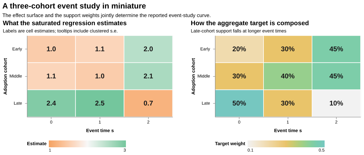{#fig-miniature-data width=100%}[Open the interactive miniature-data figure](figtab/partial_pooling_miniature_data.html).The left panel has an evident low-dimensional pattern: the early and middlecohorts are similar, their first two effects are nearly flat, and the latecohort follows a different path. The right panel shows why cohort structure canmatter for the aggregate curve. The late cohort receives 50 percent of theweight at $s=0$ and 10 percent at $s=2$. Applying the displayed weights gives$$\hat\tau_{\mathrm{sat}}=(1.73,\ 1.48,\ 1.92).$$@fig-miniature-refinement puts four restrictions on a refinement ladder.`C1-E2` uses one post-treatment rectangle. `C1-E3` splits short and long eventtimes. `C2-E3` also splits the late cohort from the early-middle block. `C3-E4`is saturated. Every move right splits an existing rectangle, and the lowerpanel maps each restricted surface back to the same support-weighted curve.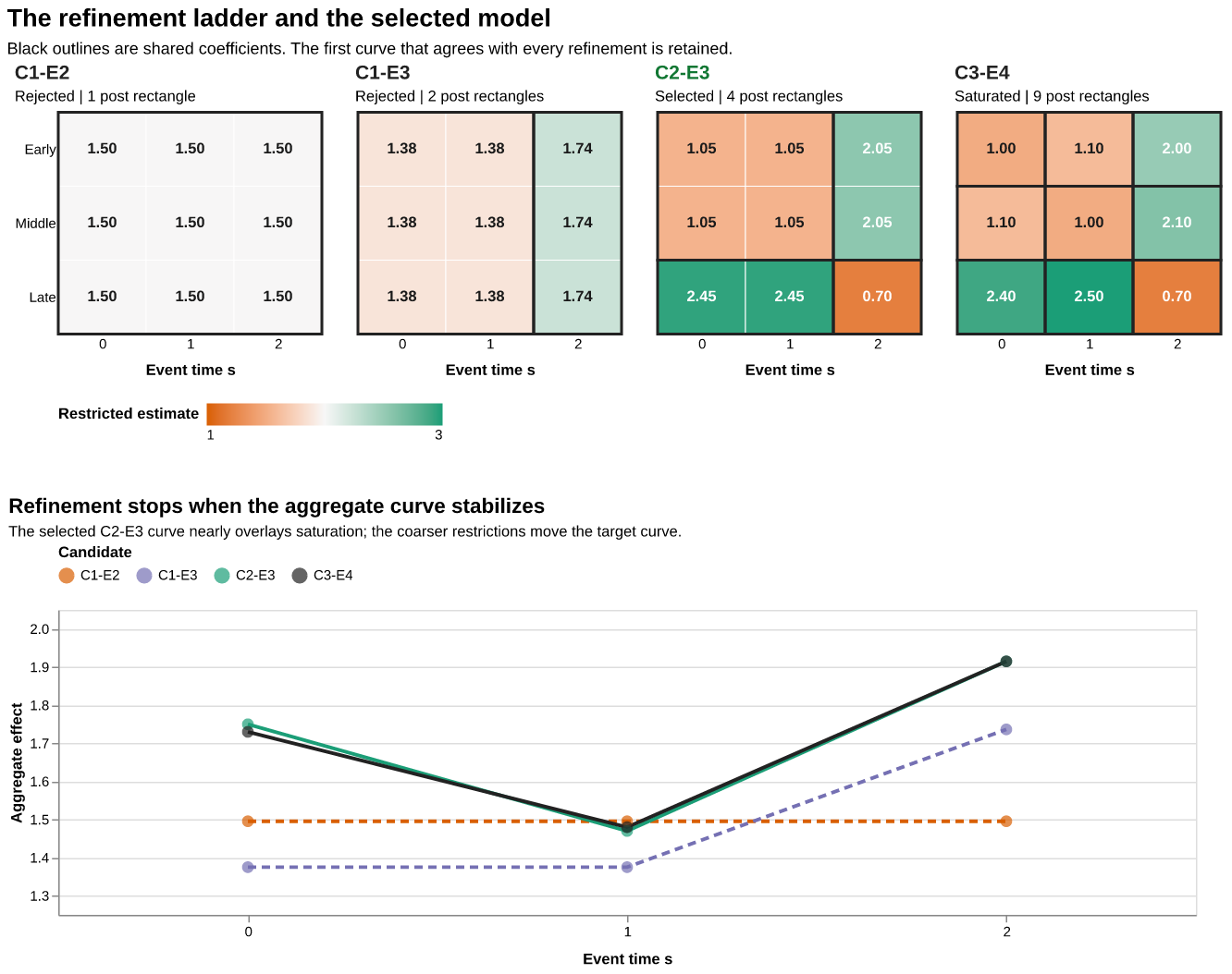{#fig-miniature-refinement width=100%}[Open the interactive refinement figure](figtab/partial_pooling_miniature_refinement.html).In this illustration, the first two restrictions visibly move the aggregatecurve. The `C2-E3` curve remains compatible with its saturated refinement, sothe rule stops there. Its four post-treatment coefficients are 1.05 and 2.45for the early-middle and late short-run blocks, and 2.05 and 0.70 for theirlong-run blocks. Applying the original target weights gives$$\hat\tau_{C2-E3}=(1.75,\ 1.47,\ 1.92),$$which nearly overlays the saturated aggregate using four post-treatmentcoefficients in place of nine. The full procedure is visible in the two figures:estimate transparent cohort-event cells, project them onto nested rectangles,map every projection to the same target, and retain the least complex curve thatagrees with all refinements. Section 3 develops the projection, comparisoncovariance, and simultaneous critical value used for that decision.## 3. Method: Adaptive Partial Pooling on a LatticeThis section develops the paper's estimator from beginning to end. Section 2delivered a saturated vector $\hat\theta$, its covariance $\hat\Sigma$, and thecommon target map $L$. The task now is to use restrictions on $\theta$ to reducevariance without silently changing $L\theta$. We first build a nested collectionof interpretable restrictions, then project every restricted estimate back tothe same target curve, use Lepskii comparisons to decide how much refinement thedata require, separate that within-lattice decision from hyperparameter tuningand inference, and finally state the formal limits of the procedure. Together,these consecutive stages form one adaptive estimator.### 3.1 Constructing candidate restrictionsThe goal of this first stage is to turn the unrestricted cohort-by-event-timesurface from Section 2 into an ordered set of plausible lower-dimensionalsurfaces. This supplies the approximation class for the paper's bias-varianceproblem: coarse members pool many cells and can be precise, while fine membersretain more heterogeneity and approach the saturated estimator. The nestingstructure introduced here is also what makes the later Lepskii comparisonsdirectional and interpretable.#### Nested adjacent partitionsStart with a toy event study containing three adoption cohorts,$g\in\{3,5,7\}$, and five reported event times,$s\in\{-2,0,1,2,3\}$. The reference period $s=-1$ is normalized away. Thecohort partitions in this example are$$\begin{aligned}\mathcal P_1 &= \bigl\{\{3,5,7\}\bigr\},\\\mathcal P_2 &= \bigl\{\{3,5\},\{7\}\bigr\},\\\mathcal P_3 &= \bigl\{\{3\},\{5\},\{7\}\bigr\},\end{aligned}$$and the event-time partitions are$$\begin{aligned}\mathcal Q_2 &= \bigl\{\{-2\},\{0,1,2,3\}\bigr\},\\\mathcal Q_3 &= \bigl\{\{-2\},\{0,1\},\{2,3\}\bigr\},\\\mathcal Q_5 &= \bigl\{\{-2\},\{0\},\{1\},\{2\},\{3\}\bigr\}.\end{aligned}$$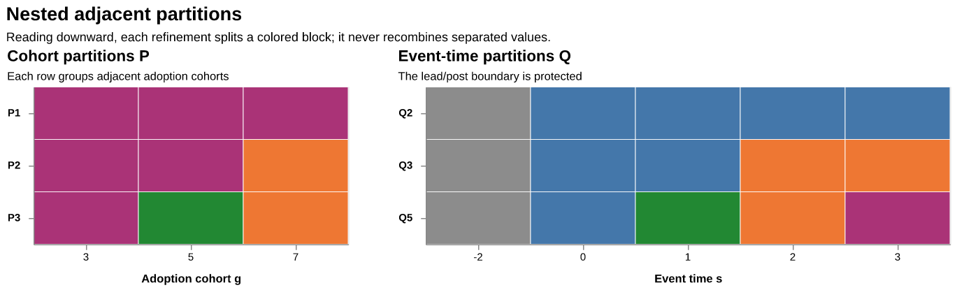{#fig-partition-paths width=100%}[Open the interactive partition figure](figtab/partial_pooling_partition_paths.html).The distinction is concrete. $\mathcal P_a$ says which neighboring adoptioncohorts must share coefficients. $\mathcal Q_b$ says which neighboring eventtimes must share coefficients. For example, $\mathcal P_2$ allows the latecohort to differ from the early and middle cohorts, while $\mathcal Q_3$ allowsthe lead, short-run response, and long-run response to differ.A finer partition splits existing blocks, and every finer block remains insideone coarser block. Thus $\mathcal Q_3$ refines $\mathcal Q_2$ because each blockof $\mathcal Q_3$ lies entirely inside a block of $\mathcal Q_2$. Theimplementation constructs each path recursively to preserve this containment.Independent equal-width binning at every dimension can violate nesting. Theprotected break at zero keeps leads and lags in separate blocks.#### Crossing partitions into coefficient rectanglesCrossing a cohort partition with an event-time partition turns the twoone-dimensional groupings into a restricted treatment-effect surface. In thetoy truth below, the early and middle cohorts share a path, the late cohort hasa different path, and the post-treatment response has short- and long-runphases. The middle candidate, $\mathcal P_2\times\mathcal Q_3$, therefore matchesthe six true coefficient rectangles exactly.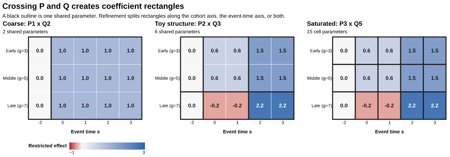{#fig-partition-rectangles width=100%}[Open the interactive coefficient-rectangle figure](figtab/partial_pooling_partition_rectangles.html).The left panel pools all post-treatment cells into one coefficient. The middlepanel splits both axes just enough to recover the toy structure. The right panelassigns a separate coefficient to every displayed cohort-event cell. Arefinement may split rectangles along the cohort axis, the event-time axis, orboth. It weakens restrictions and raises dimension.Formally, candidate $m=(a,b)$ imposes equality within rectangles of$\mathcal P_a\times\mathcal Q_b$. Let $H_m$ be the $p\times d_m$ expansionmatrix satisfying$$\theta=H_m\eta_m$$when the restriction is exact. With incomplete support, $H_m$ contains rows forcells in $\mathcal I$, and parameters correspond to nonempty rectangles.The partial order is$$m\preceq f\quad\Longleftrightarrow\quad\mathcal P_f\text{ refines }\mathcal P_m\text{ and }\mathcal Q_f\text{ refines }\mathcal Q_m.$$This containment relation organizes the candidates as a lattice. We label acandidate with $K$ cohort blocks and $R$ event-time blocks as$C_K\text{-}E_R$; for example, the middle toy model is `C2-E3`.### 3.2 Mapping every candidate to the common targetThe partitions above describe restrictions on the cohort-event surface. Thereported object is an aggregate event-study curve. This stage turns eachcandidate restriction into an estimator of the same $\tau=L\theta$ defined inSection 2. Holding the target fixed ensures that differences between coarse andfine models measure the consequences of pooling under one common estimand.#### Minimum-distance projectionIt helps to keep the three spaces separate. The vector $\eta_m$ contains onecoefficient per nonempty rectangle, $\theta$ contains one coefficient persupported cohort-event cell, and $\tau$ contains one coefficient per reportedevent time. The matrices below move between those spaces.| Object | Dimension | Role ||---|---:|---|| $H_m$ | $p\times d_m$ | expands $d_m$ rectangle coefficients into $p$ supported cells || $P_m$ | $p\times p$ | replaces a saturated cell surface by its restricted fitted surface || $L$ | $q\times p$ | aggregates supported cells into the fixed $q$-period target curve || $D_m=LP_m$ | $q\times p$ | maps the saturated estimate directly to candidate $m$'s target curve |For positive semidefinite metric $W$, estimate the restricted parameters by$$\hat\eta_m=(H_m'WH_m)^+H_m'W\hat\theta,$$where $+$ denotes a Moore-Penrose inverse. Define$$P_m=H_m(H_m'WH_m)^+H_m'W.$$The first equation chooses the rectangle coefficients whose expanded surface$H_m\eta_m$ is closest to $\hat\theta$ in the geometry defined by $W$. The secondcollects that calculation into the projection map $P_m$. The same basefixed-effects regression supplies every candidate.The fitted surface and common target curve are$$\hat\theta_m=P_m\hat\theta,\qquad\hat\tau_m=LP_m\hat\theta=D_m\hat\theta.$$Thus $\hat\theta_m$ is useful for inspecting the restricted cohort-time surface,whereas $\hat\tau_m$ is the object compared and ultimately reported. Every$\hat\tau_m$ has the same coordinates and target weights; only the amount ofpooling used to estimate it changes.The production estimator uses feasible GLS, $W=\hat\Sigma^+$. If model $m$ iscorrect, this is the efficient minimum-distance estimator under the saturatedGaussian approximation. Under misspecification, it estimates a projection:$$\theta_m^{\mathrm{proj}}=P_m\theta,\qquadB_m=LP_m\theta-L\theta.$$This projection bias is the cost of pooling.A support-weighted projection is also available as a diagnostic. When the samesupport weights define both the within-event-time projection and $L$, cohortpooling leaves the aggregate target numerically invariant and offers nomeaningful variance gain for that target. GLS weighting converts the equalityrestrictions into an efficiency gain under the restricted model, with anexplicit bias cost away from it.#### Joint covariance across candidatesThe next selection stage compares candidate curves to one another and thereforerequires the covariance of their difference in addition to each curve's marginalstandard errors. All candidates are transformations of the same saturatedestimate and are highly correlated; preserving that dependence is one of themain practical benefits of constructing the entire lattice from one base fit.Conditional on the estimated projection matrices,$$\widehat{\operatorname{Var}}(\hat\tau_m)=D_m\hat\Sigma D_m',$$and, crucially,$$\widehat{\operatorname{Cov}}(\hat\tau_m,\hat\tau_f)=D_m\hat\Sigma D_f'.$$Thus the covariance of a model difference is$$\hat S_{m,f}=(D_m-D_f)\hat\Sigma(D_m-D_f)'.$$Adding the two marginal variances would ignore their common saturated fit andsubstantially overstate comparison noise.#### Endpoints and the external comparatorThe lattice contains several familiar restrictions:- one cohort block with saturated event time is a common-cohort dynamic curve;- one lead block and one post block with one cohort block is a static pooled restriction, subject to the lead normalization;- saturated cohorts and saturated event times reproduce $\hat\theta$ exactly;- intermediate rectangles represent adoption regimes and dynamic phases.The common-cohort minimum-distance endpoint differs algebraically from a naiveTWFE event study. The simulations estimate naive TWFE in a separate regressionand use it as an external comparator outside the lattice.### 3.3 Choosing complexity with Lepskii comparisonsThe preceding stages produce many estimates of one target curve: coarsecandidates have lower sampling variance when their restrictions are adequate,whereas fine candidates are less exposed to pooling bias. This stage decideswhich precision gains the data support. Its role in the overall paper is to turnthe candidate lattice from a menu that a researcher must choose manually intoan estimator with a reproducible data-dependent complexity choice.The selector asks whether relaxing a coarse candidate's restrictions changes thereported target curve by more than can be explained by the shared sampling noisein $\hat\theta$. This target-specific comparison allows pooling when latentheterogeneity aggregates away and triggers refinement when heterogeneitymaterially changes the aggregate target.Lepskii's principle answers that question by starting from the precision-favoringend of the lattice. A candidate remains viable only if its curve agrees with allof its finer, less restricted comparators after accounting for uncertainty. Theselected model is the least complex viable candidate. This implements aone-sided burden of proof: additional parameters are retained only when arefinement reveals a target-relevant discrepancy.#### Pairwise target-curve discrepanciesFor a coarse candidate $m$ and a comparable refinement $f\succeq m$, define$$\hat\Delta_{m,f}=\hat\tau_m-\hat\tau_f.$$At the population level the corresponding difference is$$\Delta_{m,f}=L(P_m-P_f)\theta.$$If the restriction imposed by $m$ is adequate for the target, both candidateshave the same target limit and $\Delta_{m,f}=0$. If pooling in $m$ distorts thetarget, at least one refinement can produce a nonzero difference. We compareonly nested pairs because $f\succeq m$ has a precise meaning: $f$ relaxes someof the equalities imposed by $m$ and imposes none that conflict with them.Each incomparable candidate receives its own refinement checks. Directspecification comparisons use nested pairs.Section 3.2 supplied the covariance $\hat S_{m,f}$ of the difference. For eachevent time, the standardized discrepancy is therefore$$Z_{m,f,s}=\frac{\hat\Delta_{m,f,s}}{\sqrt{\hat S_{m,f,ss}}}.$$The implementation summarizes the entire curve comparison by its largestabsolute standardized discrepancy on a prespecified selection set$\mathcal S_0$:$$T_{m,f}=\max_{s\in\mathcal S_0}\left|\frac{\hat\Delta_{m,f,s}}{\sqrt{\hat S_{m,f,ss}}}\right|.$$Large $T_{m,f}$ means that some target coordinate changes too much to attributeto estimation noise; small $T_{m,f}$ supports retaining the coarser candidate.The default $\mathcal S_0$ contains supported post-treatment event times andexcludes the normalized reference period and the weakest tail. This set is partof the scientific decision: it identifies the portion of the curve whoseapproximation quality governs pooling. The reported curve may include additionalevent times.Every finer model contributes information to the comparison. A noisy saturatedcurve can mask a departure that is visible in a well-chosen intermediaterefinement. For example, in the toy surface, a cohort split can reveal the latecohort's different response before every cohort-event cell is estimatedseparately. The rule therefore compares each candidate with every finer memberof the lattice.#### Simultaneous cluster multiplier calibrationThe statistic above is searched over event times, over refinements of a givencandidate, and ultimately over all candidates considered for selection. Apointwise normal cutoff yields excessive rejection under this search. Onecluster multiplier process approximates the joint null distribution of theentire family.For draw $r$, generate independent cluster multipliers $\xi_c^{(r)}$ with meanzero and variance one. The perturbation of the saturated vector is$$\hat\theta^{*(r)}-\hat\theta=\sum_c\xi_c^{(r)}\hat\psi_c.$$The same multiplier draw is passed through every candidate difference,$$\hat\Delta_{m,f}^{*(r)}=(D_m-D_f)\sum_c\xi_c^{(r)}\hat\psi_c.$$Reusing the draw is important: it preserves the dependence across models andevent times induced by their common saturated fit. After standardization by$\hat S_{m,f,ss}^{1/2}$, let $Z^{*(r)}$ be the maximum absolute perturbation overall comparable $(m,f)$ pairs and all $s\in\mathcal S_0$. The critical value isthe empirical $1-\alpha$ quantile,$$\hat c_{1-\alpha}=Q_{1-\alpha}\{Z^{*(r)}\}_{r=1}^R.$$This one threshold accounts jointly for the event-time maximum, everyrefinement comparison, and the fact that acceptance is checked for multiplecandidate models. The bootstrap is used here to calibrate the selection rule;Section 3.4 develops uncertainty statements for the selected treatment-effectcurve.#### Acceptance and model choiceCandidate $m$ is accepted when$$T_{m,f}\leq\hat c_{1-\alpha}\quad\text{for every }f\succeq m.$$Acceptance records statistical agreement with every permitted relaxation at thetarget-curve level. Surface-level equality remains unassessed. The saturatedmodel is accepted vacuously because its refinement set is empty, which guaranteesat least one accepted candidate.Among accepted candidates, the procedure selects the model with the fewestestimable rectangles. Ties are resolved by fewer cohort blocks, then fewerevent-time blocks, then lower estimated target variance. In the toy example,the coarse $\mathcal P_1\times\mathcal Q_2$ candidate should fail once its pooledcurve is compared with refinements that isolate the late cohort and the dynamicphases. If $\mathcal P_2\times\mathcal Q_3$ then agrees with every finer curve,the rule stops there and avoids the variance cost of fifteen saturated cells.The full within-lattice procedure can be read as six operations:1. Fit the saturated surface once and recover $\hat\theta$, $\hat\Sigma$, and cluster influence contributions $\hat\psi_c$.2. Build each candidate map $D_m=LP_m$ and its common-target curve $\hat\tau_m=D_m\hat\theta$.3. For every nested pair, compute $\hat\Delta_{m,f}$ and its shared-fit covariance $\hat S_{m,f}$.4. Use common multiplier draws to obtain one simultaneous critical value.5. Retain candidates that agree with every finer comparator.6. Report the least complex retained candidate as $\hat m$ and its curve as $\hat\tau_{\hat m}$.### 3.4 Tuning the procedure and reporting uncertaintySection 3.3 selects a model inside a specified lattice, conditional on choicessuch as the partition path, projection metric, and selection level. This stageaddresses a different problem: how those procedural choices are set and whatuncertainty statement is attached to the resulting curve. Keeping the twolayers separate is necessary for the paper's adaptive goal. A simultaneouscutoff accounts for searching within one lattice. Searching across alternativelattices requires independent validation.#### What is fixed and what is tunedThe procedure separates three classes of choices.| Class | Examples | Rule ||---|---|---|| Structural | target weights, comparison group, reference period, event window, adjacency, protected pre/post break, selection loss | fixed before examining outcomes || Candidate-grid | cohort path, event-time path, balanced versus front-loaded partition basis, minimum block support, projection metric | tuned only by honest validation || Calibration | selection level $\alpha$, multiplier distribution, bootstrap draws | fixed for the primary specification; varied in sensitivity analysis |The minimum cell support that defines the target is structural. The minimumsupport allowed for an intermediate pooled rectangle can be tuned because itchanges the candidate grid without changing $L\theta$.The implemented basis-family comparison remains within nested piecewise-constantmodels. The balanced family bisects the largest available block; thefront-loaded family uses narrower early post-treatment blocks before allocatingresolution to the tail. Splines or other nested smooth bases can enter throughthe same $H_m$ interface. The reported experiment uses the twopiecewise-constant families.This classification prevents tuning from redefining the scientific question.Structural choices determine the estimand or identifying design and are fixed.Candidate-grid choices determine which bias-variance compromises the selectormay consider and can be ranked by independent predictive evidence. Calibrationchoices govern the conservativeness and numerical accuracy of the search andare prespecified for the primary analysis.#### Honest nested cluster splittingThe tuning objective is the risk of the *whole adaptive procedure* under ahyperparameter configuration $h$. Each training fold therefore runs thecomplete procedure from Section 3.3, including its own multiplier calibrationand model choice. An independent saturated estimate from the validation foldsupplies a restriction-free target benchmark with sampling noise.Clusters are stratified by adoption cohort, including the never-treated group.An outer split reserves one set of clusters exclusively for inference. Theremaining clusters are divided into inner folds. For hyperparameterconfiguration $h$ and validation fold $v$, fit the adaptive estimator on thetraining folds and estimate the saturated target independently in fold $v$.For fixed event-time weights $a_s$, use the noise-corrected loss$$\widehat R_{h,v}=\sum_{s\in\mathcal S_0}a_s\left[(\hat\tau_{h,-v,s}-\hat\tau_{\mathrm{sat},v,s})^2-\widehat{\operatorname{Var}}(\hat\tau_{\mathrm{sat},v,s})\right].$$The subtraction has a direct purpose. Conditional on the training estimate andignoring fold-to-fold target drift,$$E\left[(\hat\tau_{h,-v,s}-\hat\tau_{\mathrm{sat},v,s})^2\mid \hat\tau_{h,-v,s}\right]=(\hat\tau_{h,-v,s}-\tau_s)^2+\operatorname{Var}(\hat\tau_{\mathrm{sat},v,s}).$$Because training and validation clusters are independent, subtracting thevalidation variance removes this noise floor and leaves the target risk of thetraining procedure in expectation. Stratification keeps the fold targetpopulations as similar as possible; remaining differences in support are asource of approximation error. The implementation usesinverse-validation-variance weights by default to limit the influence of weaklyestimated validation coordinates, and reports equal-weight sensitivity.Each training fit calibrates its own pathwise multiplier critical value. Afterinner validation chooses a configuration, that configuration is fit on the fulltuning sample to select one lattice model. The resulting model key is then heldfixed and estimated on the untouched outer inference sample. Hyperparameters andthe model key depend exclusively on the tuning clusters and validation loss.The outer split adds an independent inference layer to cross-validation. Itcreates a final sample on which both the hyperparameters and the discrete modelchoice are predetermined. This clean separation of model construction anduncertainty calculation costs precision.#### Three levels of inferenceThe preceding selection and tuning steps create several possible meanings of astandard error. The software separates precision gains from pooling, protectionagainst model selection, and protection against projection bias into threeinferential objects.1. **Model conditional.** Treat the selected model as fixed and use $D_{\hat m}\hat\Sigma D_{\hat m}'$. These intervals provide model-conditional diagnostics. Unconditional post-selection coverage requires an additional adjustment.2. **Honest split sample.** Use the tuning clusters to select hyperparameters and a model, then estimate on the outer inference sample. Conditional intervals are honest with respect to the tuning and model-selection stage, at a direct efficiency cost. They cover the original target $L\theta$ only when the fixed selected model's projection bias is negligible. Projection bias persists after sample splitting.3. **Bootstrap after selection.** On the full sample, perturb the saturated estimate with cluster multipliers, rerun selection in every draw, and form percentile intervals from selected curves. This captures discrete model selection conditional on the observed projection matrices. The implementation holds those matrices fixed in each draw, yielding an empirical selection adjustment. Uniformly valid confidence bands require stronger theory.### 3.5 What the method guaranteesThe previous stages define the complete estimator and its inferential variants.This final part of the method section states the scope of the formal claims. Theresults explain why candidate curves have tractable joint limits and when theselector removes overly coarse models. The claims cover a fixed finite lattice.Adaptive minimaxity over a growing nonparametric class and uniformly validfull-sample post-selection inference remain open.#### AssumptionsThe assumptions deliberately attach to the saturated estimator and the finitecollection of linear maps built above. They allow the partial-pooling machineryto inherit identification and asymptotic normality without imposing a separatedata-generating model for every candidate.**Assumption A (identified saturated limit).** Under no anticipation, paralleltrends, and overlap, $\hat\theta\overset p\to\theta$ for the supported cells.**Assumption B (joint linearity).** The saturated estimator has a cluster-levelasymptotic linear representation, $\hat\Sigma$ is consistent, and relevantcontrast variances are bounded away from zero after removing deterministicnormalizations.**Assumption C (finite nested lattice).** The cohort and event-time paths arefinite, deterministic, and nested. The target map $L$ and selection set$\mathcal S_0$ are fixed.**Assumption D (bootstrap validity).** The cluster multiplier processconsistently approximates the joint Gaussian limit of all standardized$(m,f,s)$ contrasts.#### Proposition 1: candidate limitsThe first result identifies the estimand of each restricted candidate. It makesthe source of any pooling bias explicit and links the projection in Section 3.2to the common target used by selection.For fixed $m$, if $\hat W\overset p\to W$, then$$\hat\tau_m\overset p\longrightarrowLP_m(W)\theta.$$If $\theta\in\operatorname{col}(H_m)$, then $P_m(W)\theta=\theta$ and$\hat\tau_m$ is consistent for $L\theta$. Otherwise its probability limit hastarget bias $B_m=L[P_m(W)-I]\theta$.#### Proposition 2: joint covarianceThe second result establishes a joint law for the whole candidate path. It isthe formal basis for the difference covariance $\hat S_{m,f}$ and the commonmultiplier process.For any finite set of candidates,$$\sqrt n\begin{pmatrix}\hat\tau_{m_1}-LP_{m_1}\theta\\\vdots\\\hat\tau_{m_K}-LP_{m_K}\theta\end{pmatrix}\rightsquigarrowN(0,\Omega),$$where block $(k,l)$ of $\Omega$ is$D_{m_k}\Sigma D_{m_l}'$. This follows by applying a finite collection oflinear maps to the saturated influence function. Feasible GLS contributes onlyhigher-order error under consistency and regularity of $\hat W$.#### Proposition 3: exact-structure selectionThe third result describes the clean benchmark in which one candidate is thelowest-dimensional adequate representation of the target. It formalizes theselector's intended behavior in the exact block designs used later as diagnosticfinger exercises.Let $m_0$ be the lowest-complexity candidate whose target limit equals the targetand whose finer candidates share that target limit. Suppose every lower-complexity candidate has at least one comparable refinement and event time forwhich the standardized population contrast diverges, while Assumptions A-Dhold. Then the simultaneous rule rejects every lower-complexity candidate withprobability approaching one and accepts $m_0$ with probability at least$1-\alpha+o(1)$. With a vanishing selection level satisfying the usual powercondition, selection of $m_0$ is consistent.Approximate structure is empirically central. When every candidate is anapproximation, bias and variance jointly determine the desirable model. Thenatural oracle is$$m^*=\arg\min_{m\in\mathcal M}\left\{B_m'AB_m+\operatorname{tr}(A D_m\Sigma D_m')\right\},$$for reporting loss $A$. A sharp oracle inequality on the two-dimensionalpartial order requires additional monotonicity linking target bias andrefinement. Without that monotonicity, the theoretical claim stops at exactstructure. The numerical study reports regret relative to the best feasiblelattice candidate under repeated-sample risk.## 4. ImplementationSection 3 defines the estimator as a sequence of partitions, linear projections,joint comparisons, tuning decisions, and uncertainty calculations. This sectiontranslates those mathematical objects into the software used in the paper. Itsgoal is to present the proposed procedure as an operational pyfixest extensionfor applications and simulations, and to identify the diagnostics exposed to anapplied user before the numerical evaluation begins.`LepskiiEventStudy` subclasses pyfixest's `DID` interface. One saturated pyfixestfit supplies coefficients, CRV1 covariance, residualized scores, and the bread.The implementation verifies numerically that the cluster influence stackreproduces the pyfixest covariance before using it for calibration.```{python}#| eval: falsefrom lepskii import LepskiiEventStudyfit = LepskiiEventStudy( data=df, yname="outcome", idname="unit_id", tname="period", gname="first_treated", event_grid=range(-5, 13), selection_event_times=range(0, 12), cohort_bins=[1, 2, 3, 5, "saturated"], event_time_bins=[2, 3, 5, 9, "saturated"], event_partition_strategy="balanced", threshold=None, bootstrap_draws=999, projection_weights="gls",).estimate()fit.summary()fit.target_curve()fit.selection_adjusted_tidy(draws=999)```The result object exposes all candidate curves, the acceptance lattice,pairwise statistics, selected partitions, unsupported cells, and conditional oradjusted intervals. `LepskiiTuner` implements the stratified outer split andinner noise-corrected risk comparison. Tests cover partition nesting, protectedbreaks, target mappings, unsupported cells, covariance reconstruction, bothoracle endpoints, calibration reproducibility, honest cluster separation, andAltair schema validation.## 5. Numerical ExperimentThe preceding section establishes how the estimator is computed. This sectionconstructs a controlled many-small-cohort experiment to determine whether thosecomputations solve the paper's substantive problem: retaining precision whenpooling restrictions are useful and moving toward saturation as thoserestrictions fail.It first defines the treatment-effect surfaces and candidate lattice, then fixesthe competing estimators and repeated-sample criteria used in the results.### 5.1 DesignThe experiment uses $T=36$ periods and nine treated cohorts adopting in periods$8,10,\ldots,24$. Cohort shares are uneven and sum to 0.82; the remaining unitsare never treated. The main run uses $n=1{,}200$ units and 50 replications perDGP. Unit, time, and serially correlated idiosyncratic shocks are generated bythe repository's existing panel DGP utility.The cohort path is$$K\in\{1,2,3,5,9\},$$and the event-time path is$$R\in\{2,3,5,9,17\}.$$The 17-bin endpoint separates every reported nonreference event time. Selectionuses lags $0$ through $11$ and 399 Rademacher cluster multiplier draws. The samenumber of draws is used for bootstrap-after-selection intervals.The suite includes exact finger exercises and less favorable patterns:- complete homogeneity, with oracle candidate `C1-E2`;- three cohort-only blocks, aligned with `C3-E2`;- a common short-versus-long response, aligned with `C1-E3`;- an early/late long-run interaction, aligned with `C2-E5`;- smooth gradients, delayed responses, local shocks, and F-test-style log, shark-fin, and sinusoidal curves;- three designs in which every cohort has a distinct path.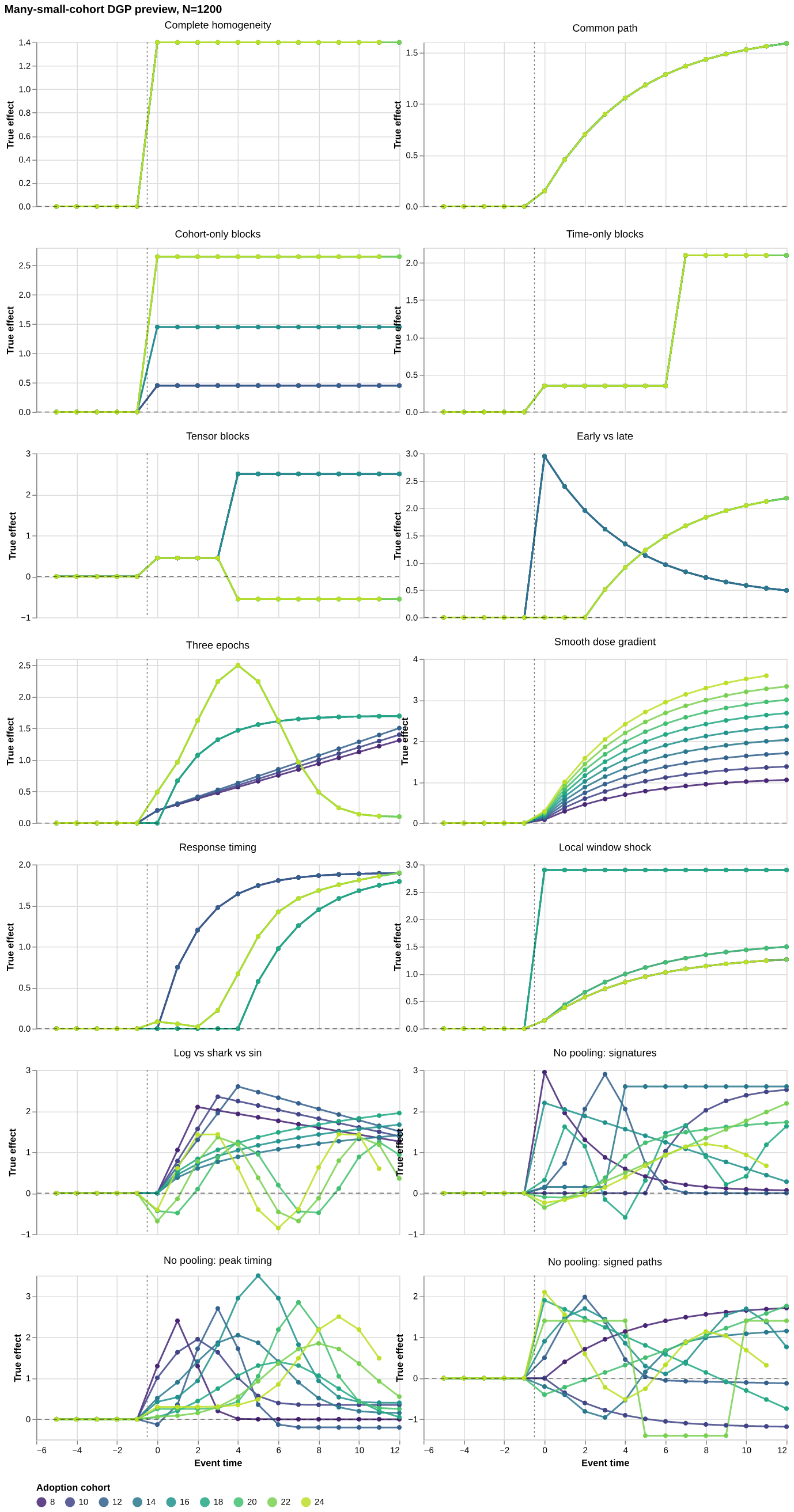{#fig-dgp-truth width=100%}[Open the interactive DGP figure](figtab/partial_pooling_dgp_truth.html).### 5.2 Estimators and metricsEvery method reports a curve on the event-time grid $s=-5,\ldots,12$, with$s=-1$ normalized to zero. MSE and bias use the post-treatment selection window$s=0,\ldots,11$ and the true support-weighted aggregate $\tau_s$ as thereference. The figures and tables use the following six estimator labels.1. **Naive TWFE.** This is a separately estimated pooled event-study regression with unit fixed effects, period fixed effects, and one relative-time coefficient shared by all treated cohorts. The reference period is $s=-1$ and standard errors cluster by unit. Under cohort heterogeneity, its coefficient can differ from the support-weighted target $\tau_s$.2. **Fixed intermediate.** This is the `C3-E5` lattice candidate in every DGP and replication: three adjacent cohort blocks crossed with five adjacent event-time blocks. Its curve is $D_m\hat\theta$ for model key `C3-E5`, using the balanced partition path and feasible GLS projection. It measures the performance of a plausible amount of partial pooling fixed before seeing outcomes.3. **Lepskii selected.** This is the primary full-sample adaptive estimator. It searches the balanced lattice with cohort counts $K\in\{1,2,3,5,9\}$ and event-time counts $R\in\{2,3,5,9,17\}$, calibrates the simultaneous rule with 399 Rademacher cluster multiplier draws, and reports the least complex accepted candidate. Selection and estimation use the same replication sample.4. **Honest tuned.** This procedure reserves half of the unit clusters for final inference. Two-fold noise-corrected validation on the tuning half ranks four prespecified lattice configurations, including balanced and front-loaded paths. The winning configuration runs Lepskii on the full tuning half, and the resulting model key is estimated on the untouched inference half. This computationally intensive comparator is run for ten replications per DGP.5. **Saturated.** This is the `C9-E17` lattice endpoint, with one parameter for every supported cohort-event cell. Its reported curve aggregates the saturated cell estimates with the same matrix $L$ used by every lattice candidate. It is the finest fixed candidate and carries the highest sampling variance when the surface admits pooling.6. **Oracle feasible.** For each DGP, we compute the repeated-sample post-treatment MSE of every fixed lattice candidate and choose one model key with the lowest MSE. That same model key is evaluated in every replication of the DGP. The oracle uses the completed Monte Carlo experiment and serves as a fixed-candidate risk benchmark.The oracle benchmark can lie above an adaptive estimator because Lepskii maychoose different candidates in different samples. Naive TWFE can also attain alower estimated MSE because it lies outside the lattice. Monte Carlo error canproduce small negative estimated regret.For estimator $a$ and DGP $d$,$$\operatorname{MSE}_{d,a}=\frac{1}{|\mathcal S_0|}\sum_{s\in\mathcal S_0}E[(\hat\tau_{d,a,s}-\tau_{d,s})^2].$$Oracle regret is MSE minus the feasible-oracle MSE. We also report squared bias,variance, pointwise coverage, interval length, selection frequencies, andruntime.```{python}#| label: load-resultsfrom pathlib import Pathimport pandas as pdresult_dir = Path("figtab")metrics = pd.read_csv(result_dir /"partial_pooling_simulation_metrics.csv")oracle = pd.read_csv(result_dir /"partial_pooling_simulation_oracle.csv")selection_frequency = pd.read_csv( result_dir /"partial_pooling_simulation_selection_frequency.csv")selections = pd.read_csv(result_dir /"partial_pooling_simulation_selections.csv")selector_sensitivity = pd.read_csv( result_dir /"partial_pooling_sensitivity_summary.csv")tuning_sensitivity = pd.read_csv( result_dir /"partial_pooling_sensitivity_tuning_summary.csv")```## 6. ResultsSection 5 fixes the DGPs, estimators, and evaluation criteria; this section usesthem to assess the adaptive estimator against the paper's overall objective. Theevidence is organized from visual behavior to repeated-sample risk, selectedcomplexity, interval performance, sensitivity, and computation. Reading theseobjects together evaluates risk, the plausibility of selected structures, andthe reliability of uncertainty statements.The representative-curve figure displays naive TWFE, full-sample Lepskii, andthe saturated aggregate because those three curves expose the pooled,data-adaptive, and fully heterogeneous behaviors in one replication. The riskfigure and MSE table compare naive TWFE, the fixed `C3-E5` candidate,full-sample Lepskii, honest tuned Lepskii, the saturated `C9-E17` endpoint, andthe repeated-sample feasible oracle. The selection-frequency figure describesthe model keys chosen by full-sample Lepskii. The coverage figure reportsmodel-conditional intervals for naive TWFE, fixed `C3-E5`, full-sample Lepskii,honest tuned Lepskii, and saturated `C9-E17`; its interactive tooltips alsoreport selection-adjusted intervals for full-sample Lepskii.### 6.1 Representative event-study curves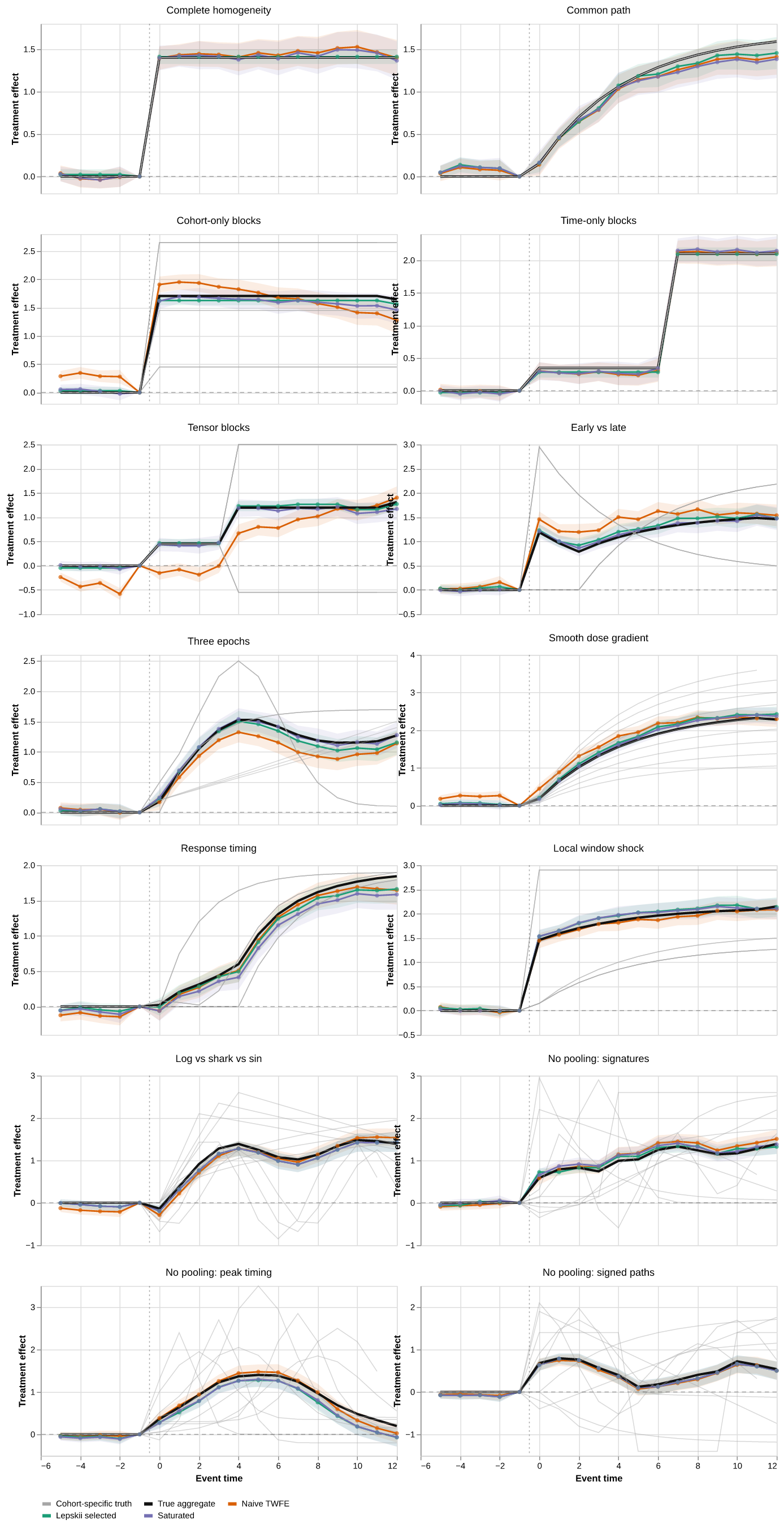{#fig-curves width=100%}[Open the interactive event-study figure](figtab/partial_pooling_simulation_curves.html).The line legend is deliberately separate from the translucent ribbons: lightgray denotes latent cohort-specific paths, black the true aggregate target,orange naive TWFE, green the Lepskii-selected curve, and purple the saturatedcurve. These representative draws illustrate one selected model. The risk andcoverage comparisons below use all available replications.### 6.2 Risk and oracle regret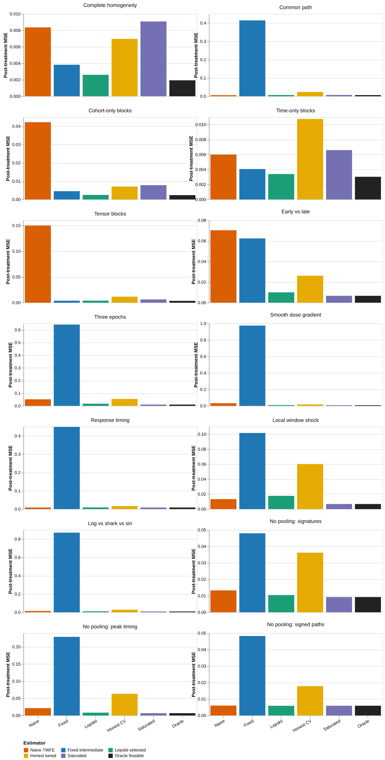{#fig-risk width=100%}[Open the interactive risk figure](figtab/partial_pooling_simulation_risk.html).```{python}#| label: tbl-mse#| tbl-cap: "Post-treatment MSE relative to the best feasible lattice candidate."mse_table = ( metrics.pivot_table( index="dgp_label", columns="estimator", values="mse_over_oracle", ) .reindex( columns=["Naive TWFE","Fixed intermediate","Lepskii selected","Honest tuned","Saturated","Oracle feasible", ] ) .round(2))mse_table.rename_axis(index="DGP", columns=None).style.format(precision=2)```The aligned designs provide the cleanest diagnostic. Complete homogeneity shouldfavor the smallest model; cohort-only heterogeneity should refine only thecohort axis; time-only heterogeneity should refine only event time; and thetensor design should refine both. The larger suite then measures how much riskis lost when the true surface is smooth, local, or misaligned with rectangles.The modal choices in those four diagnostics are, respectively, `C1-E2` in 88%of replications, `C3-E2` in 86%, `C1-E3` in 90%, and `C2-E5` in 96%. TheirLepskii MSE ratios relative to the best fixed candidate are 1.35, 1.06, 1.12,and 1.13. Thus the selector reads both axes correctly in the exact blockexperiments, although selection noise leaves a visible cost even under completehomogeneity.```{python}#| label: tbl-oracle#| tbl-cap: "Best feasible lattice model under repeated-sample post-treatment risk."oracle[ ["dgp_label", "latent_type", "oracle_model", "oracle_mse"]].rename( columns={"dgp_label": "DGP","latent_type": "Latent heterogeneity","oracle_model": "Oracle model","oracle_mse": "Oracle MSE", }).style.hide(axis="index").format({"Oracle MSE": "{:.5f}"})```### 6.3 What the selector chooses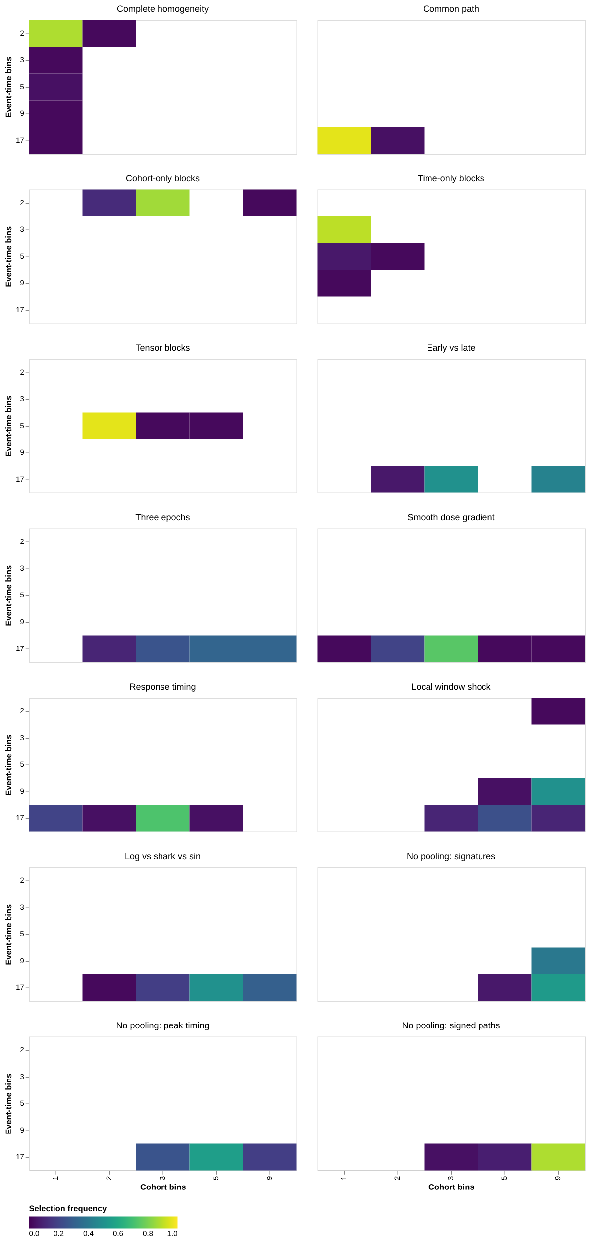{#fig-selection width=100%}[Open the interactive selection figure](figtab/partial_pooling_simulation_selection.html).```{python}#| label: tbl-selection#| tbl-cap: "Modal selected model and its frequency by DGP."modal_selection = ( selection_frequency.sort_values( ["dgp", "frequency", "selected_model"], ascending=[True, False, True], ) .groupby("dgp", as_index=False) .first())modal_selection[ ["dgp_label","selected_model","selected_cohort_bins","selected_event_bins","frequency", ]].rename( columns={"dgp_label": "DGP","selected_model": "Model","selected_cohort_bins": "Cohort bins","selected_event_bins": "Event-time bins","frequency": "Frequency", }).style.hide(axis="index").format({"Frequency": "{:.3f}"})```Selection is target-specific. In a design with a unique path for every cohort,the oracle may still pool event times if each path has exploitable temporalstructure. More subtly, the selector can pool cohorts when their projectionbias cancels in the weighted aggregate curve. Such a result supports pooling forthe aggregate target and leaves latent cohort homogeneity unresolved. Finercohort resolution delivered too little target improvement to justify itsvariance.The three deliberately non-poolable designs move sharply toward the saturatedcohort axis: their modal models are `C9-E17`, `C5-E17`, and `C9-E17`, and theirLepskii MSE ratios are 1.13, 1.23, and 0.99. The modal `C5-E17` choice in themiddle design retains some cohort pooling, consistent with selection for anaggregate curve. In the signed-path design, the adaptive selector switches amongfixed candidates across samples, so its MSE can fall below the best single fixedcandidate.### 6.4 Coverage and interval length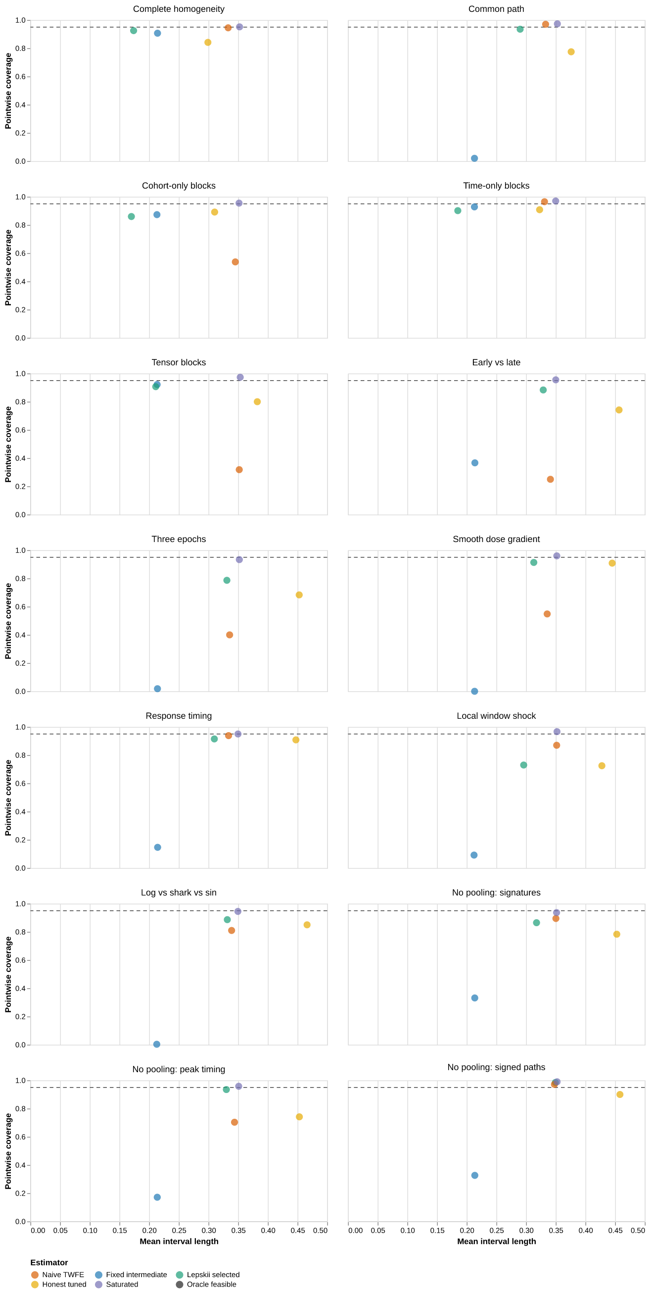{#fig-coverage width=100%}[Open the interactive coverage figure](figtab/partial_pooling_simulation_coverage.html).Model-conditional intervals are shortest in heavily pooled models. Materialprojection bias and same-sample selection can produce undercoverage.Bootstrap-after-selection intervals are generally wider. Their reported coverageserves as an empirical selection-adjustment diagnostic; uniform validity remainsopen.The localized-shock design is the clearest warning. Lepskii risk is 2.61 timesthe fixed-candidate oracle and conditional pointwise coverage is 0.73. Thebootstrap-after-selection interval raises coverage to 0.965 while increasingmean length from 0.296 to 0.421. Uniform validity remains open. Honest tuninguses only ten replications per DGP and pays heavily forthe outer half-sample: its MSE ratios range from 1.85 to 9.55. Its remainingundercoverage is consistent with projection bias that persists after independentselection.### 6.5 SensitivityThe primary selector is rerun for five replications in four representativedesigns while varying the selection level, lattice density, event-time basis,projection metric, multiplier draws, and multiplier seed. The honest tuner isrerun for three replications in the tensor and non-poolable-signature designswhile varying validation-loss weights, the number of inner folds, and the splitseed. These deliberately small runs provide stability diagnostics with limitedMonte Carlo precision.```{python}#| label: tbl-selector-sensitivity#| tbl-cap: "Sensitivity of the full-sample selector to calibration and lattice choices."selector_sensitivity_table = ( selector_sensitivity.groupby( ["axis", "scenario_label"], as_index=False, ) .agg( designs=("dgp", "nunique"), replications_per_design=("replications", "min"), model_agreement=("selection_agreement", "mean"), median_mse_over_primary=("mse_over_primary", "median"), worst_mse_over_primary=("mse_over_primary", "max"), ) .sort_values(["axis", "scenario_label"]))selector_sensitivity_table.rename( columns={"axis": "Axis","scenario_label": "Scenario","designs": "Designs","replications_per_design": "Replications","model_agreement": "Model agreement","median_mse_over_primary": "Median MSE / primary","worst_mse_over_primary": "Worst MSE / primary", }).style.hide(axis="index").format( {"Model agreement": "{:.2f}","Median MSE / primary": "{:.2f}","Worst MSE / primary": "{:.2f}", })``````{python}#| label: tbl-tuning-sensitivity#| tbl-cap: "Sensitivity of honest tuning to loss weights, folds, and split seed."tuning_sensitivity_table = ( tuning_sensitivity.groupby( ["axis", "scenario_label"], as_index=False, ) .agg( designs=("dgp", "nunique"), replications_per_design=("replications", "min"), model_agreement=("selection_agreement", "mean"), median_mse_over_primary=("mse_over_primary", "median"), worst_mse_over_primary=("mse_over_primary", "max"), ) .sort_values(["axis", "scenario_label"]))tuning_sensitivity_table.rename( columns={"axis": "Axis","scenario_label": "Scenario","designs": "Designs","replications_per_design": "Replications","model_agreement": "Model agreement","median_mse_over_primary": "Median MSE / primary","worst_mse_over_primary": "Worst MSE / primary", }).style.hide(axis="index").format( {"Model agreement": "{:.2f}","Median MSE / primary": "{:.2f}","Worst MSE / primary": "{:.2f}", })```Model agreement is the share of matched DGP-replication pairs selecting the samelattice model as the primary specification. Risk ratios compare repeated-samplepost-treatment MSE within each design before taking the reported median ormaximum across designs. The split-seed row is especially important: largemovement there signals weak information for fine hyperparameter ranking, evenwhen the outer inference step remains honest.Multiplier simulation is stable in this diagnostic: both 199 and 799 drawsmatch the primary model in every run, and the alternate multiplier seed agreesin 95% of runs. The substantive approximation choices matter more. Thefront-loaded basis agrees in 65% of runs, the coarse lattice in 20%, and theequal-weight projection in 80%; the last has a median MSE ratio of 1.35. Withinhonest tuning, equal event-time loss weights happen to agree in all six matchedruns. Three folds agree in 17%, while an alternate split seed agrees in 67% andreaches a worst-design MSE ratio of 2.59. The low replication count yieldsimprecise rankings and reveals substantial fold and split sensitivity thatbelongs alongside the tuned result.### 6.6 Computation```{python}#| label: tbl-runtime#| tbl-cap: "Mean runtime in seconds per replication."runtime_table = ( selections.groupby("dgp_label", as_index=False) .agg( lattice_fit=("fit_seconds", "mean"), selection_adjustment=("adjusted_seconds", "mean"), naive_twfe=("naive_seconds", "mean"), honest_tuning=("cv_seconds", "mean"), ) .round(2))runtime_table.rename( columns={"dgp_label": "DGP","lattice_fit": "Lattice fit","selection_adjustment": "Selection adjustment","naive_twfe": "Naive TWFE","honest_tuning": "Honest tuning", }).style.hide(axis="index").format(precision=2, na_rep="")```The lattice fit performs one fixed-effects regression regardless of the numberof candidates. Projection, comparison, and multiplier operations are denselinear algebra on the supported coefficient dimension. Honest tuning is moreexpensive because independence requires additional saturated fits on clustersubsamples.## 7. LimitationsThe results show where adaptive pooling succeeds and where local or weaklysupported heterogeneity remains difficult. This section relates those empiricalfailures back to the assumptions and design choices in Section 3 and marks theboundary of the paper's claims. Its purpose is to distinguish limitations of thecurrent candidate lattice and inferential implementation from failures of theunderlying difference-in-differences identification strategy.First, the method inherits the credibility of the saturated base estimator andits comparison group. A failed parallel-trends assumption invalidates theidentified cells before regularization begins.Second, adjacent rectangles form an interpretable, limited approximation class.A local shock that cuts across the deterministic hierarchy may require more binsthan a localized tree or fused-penalty estimator. The candidate grid thereforeembodies substantive approximation assumptions.Third, feasible GLS uses an estimated covariance metric. The reported first-order covariance treats the resulting projection matrices as fixed. This isstandard for finite-dimensional feasible minimum distance. Weakly supportedcells can make the approximation unstable, making support thresholds andcondition diagnostics essential reporting items.Fourth, the simultaneous Lepskii rule controls a family of model-differencestatistics. Unconditional confidence bands for the selected curve require anadditional inferential argument. Honest splitting is the clean default wheninferential validity is paramount. The full-sample bootstrap adjustment providesa computationally useful empirical correction, and stronger uniform theoryremains open.Finally, a target-curve selector is intentionally insensitive to latentheterogeneity that aggregates away. Researchers interested in cohort-specificeffects should select and report a surface-level loss. A coarse aggregate modelsupports a claim about the aggregate target alone.## 8. ConclusionThe limitations above delimit what can be claimed from the current theory andexperiment. This final section returns to the paper's motivating choice betweenpooled and saturated event studies, summarizes how the proposed estimatorchanges that choice, and identifies the theoretical and inferential work stillneeded to complete the broader adaptive-pooling program.Treatment effects often have low-dimensional structure across adoption cohorts,event time, or both. Theproposed estimator uses that structure without changing the reported target:start from a saturated heterogeneity-robust surface, project it onto a nestedcohort-time lattice, preserve joint covariance, and select the coarsest modelthat survives all finer comparisons.The resulting procedure turns the original joint-test diagnostic into anestimator. It recovers precision when restrictions are supported, returns towardsaturation as restrictions fail, and makes the selected structure directlyreportable. Its strongest current evidence is finite-grid implementation andsimulation performance. A general oracle inequality for approximate models on atwo-dimensional partial order and uniformly valid full-sample post-selectionbands remain the main theoretical tasks.


